Page 300 - Fair, Geyer, and Okun's Water and wastewater engineering : water supply and wastewater removal

JWCL344_ch07_230-264.qxd 8/2/10 8:44 PM Page 260

260 Chapter 7 Water Distribution Systems: Modeling and Computer Applications
under that flow pattern. Color-code the system using the ranges Table 7.19 Pump Information for Problem 7.4
given in Table 7.18. After you define the color-coding, place a
legend in the drawing (see Table 7.18). Head (ft) Head (m) Flow (gpm) Flow (L/min)
200 60.96 0 0
175 53.34 1,000 3,785
Table 7.18 Color-Coding Range for
100 30.48 2,000 7,570
Problem 7.3
Table 7.20 Junction Information for Problem 7.4
Max. Velocity
(ft/s) (m/s) Color Junction Label Demand (L/min) Demand (gpm)
0.5 0.15 Magenta J-1 1,514 400
2.5 0.76 Blue J-2 2,082 550
5.0 1.52 Green J-3 2,082 550
8.0 2.44 Yellow J-4 1,325 350
20.0 6.10 Red
Table 7.21 Pipe Information for Problem 7.4

1. Fill in or reproduce the Results Summary table after Pipe Label Length (m) Length (ft)
each run to get a feel for some of the key indicators
P-1 23.77 78
during various scenarios.
P-2 12.19 40
2. For the average day run, what is the pump discharge?
P-3 27.43 90
3. If the pump has a best efficiency point at 300 gpm P-4 11.89 39
(1,135.5 L/min), what can you say about its performance P-5 3.05 10
on an average day? P-6 3.05 10
4. For the peak hour run, the velocities are fairly low.
Does this mean you have oversized the pipes? Explain. 3. Place a check valve on pipe P-3 such that the valve
5. For the minimum hour run, what was the highest pres- only allows flow from J-3 to J-4. What happens to the
sure in the system? Why would you expect the highest flow in pipe P-3? Why does this occur?
pressure to occur during the minimum hour demand? 4. When the check valve is placed on pipe P-3, what hap-
6. Was the system (as currently designed) acceptable for pens to the pressures throughout the system?
the fire flow case with the sprinkled building? On what 5. Remove the check valve on pipe P-3. Place a 6-in.
did you base this decision? (150-mm) flow control valve (FCV) node at an eleva-
7. Was the system (as currently designed) acceptable for tion of 5 ft (1.52 m) on pipe P-3. The FCV should be set
the fire flow case with all the flow provided by hose so that it only allows a flow of 100 gpm (378.5 L/min)
streams (no sprinklers)? If not, how would you modify from J-4 to J-3. (Hint: A check valve is a pipe prop-
the system so that it will work? erty.) What is the resulting difference in flows in the
network? How are the pressures affected?
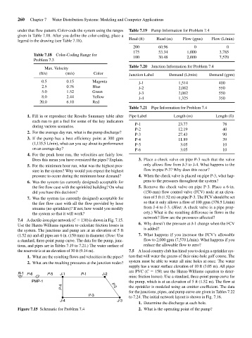
7.4 A ductile-iron pipe network (C 130) is shown in Fig. 7.15.
6. Why doesn’t the pressure at J-1 change when the FCV
Use the Hazen-Williams equation to calculate friction losses in
is added?
the system. The junctions and pump are at an elevation of 5 ft
(1.52 m) and all pipes are 6 in. (150 mm) in diameter. (Note: Use 7. What happens if you increase the FCV’s allowable
a standard, three-point pump curve. The data for the pump, junc- flow to 2,000 gpm (7,570 L/min). What happens if you
tions, and pipes are in Tables 7.19 to 7.21.) The water surface of reduce the allowable flow to zero?
the reservoir is at an elevation of 30 ft (9.14 m). 7.5 A local country club has hired you to design a sprinkler sys-
1. What are the resulting flows and velocities in the pipes? tem that will water the greens of their nine-hole golf course. The
system must be able to water all nine holes at once. The water
2. What are the resulting pressures at the junction nodes?
supply has a water surface elevation of 10 ft (3.05 m). All pipes
are PVC (C 150; use the Hazen-Williams equation to deter-
R-1 P-6 P-5 J-1 P-1 J-2
mine friction losses). Use a standard, three-point pump curve for
PMP-1 the pump, which is at an elevation of 5 ft (1.52 m). The flow at
P-4 P-2 the sprinkler is modeled using an emitter coefficient. The data
for the junctions, pipes, and pump curve are given in Tables 7.22
P-3 to 7.24. The initial network layout is shown in Fig. 7.16.
J-4 J-3
1. Determine the discharge at each hole.
Figure 7.15 Schematic for Problem 7.4 2. What is the operating point of the pump?