Page 122 - Fundamentals of Gas Shale Reservoirs

102 PORE GEOMETRY IN GAS SHALE RESERVOIRS

Image acquisition Labeling

Quanti cation

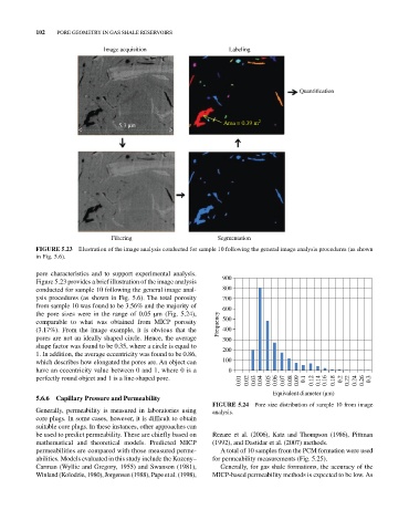
5.3 m Area = 0.39 m 2

Filtering Segmentation
FIGurE 5.23 Illustration of the image analysis conducted for sample 10 following the general image analysis procedures (as shown
in Fig. 5.6).

pore characteristics and to support experimental analysis.
Figure 5.23 provides a brief illustration of the image analysis 900
conducted for sample 10 following the general image anal­ 800
ysis procedures (as shown in Fig. 5.6). The total porosity 700
from sample 10 was found to be 3.56% and the majority of 600
the pore sizes were in the range of 0.05 µm (Fig. 5.24),
comparable to what was obtained from MICP porosity Frequency 500
(3.17%). From the image example, it is obvious that the 400
pores are not an ideally shaped circle. Hence, the average 300
shape factor was found to be 0.35, where a circle is equal to
1. In addition, the average eccentricity was found to be 0.86, 200
which describes how elongated the pores are. An object can 100
have an eccentricity value between 0 and 1, where 0 is a 0
perfectly round object and 1 is a line‐shaped pore.
0.01 0.02 0.03 0.04 0.05 0.06 0.07 0.08 0.09 0.1 0.12 0.14 0.16 0.18 0.2 0.22 0.24 0.26 0.3
Equivalent diameter ( m)
5.6.6 Capillary Pressure and Permeability
FIGurE 5.24 Pore size distribution of sample 10 from image
Generally, permeability is measured in laboratories using analysis.
core plugs. In some cases, however, it is difficult to obtain
suitable core plugs. In these instances, other approaches can
be used to predict permeability. These are chiefly based on Rezaee et al. (2006), Katz and Thompson (1986), Pittman
mathematical and theoretical models. Predicted MICP (1992), and Dastidar et al. (2007) methods.
permeabilities are compared with those measured perme­ A total of 10 samples from the PCM formation were used
abilities. Models evaluated in this study include the Kozeny– for permeability measurements (Fig. 5.25).
Carman (Wyllie and Gregory, 1955) and Swanson (1981), Generally, for gas shale formations, the accuracy of the
Winland (Kolodzie, 1980), Jorgensen (1988), Pape et al. (1998), MICP‐based permeability methods is expected to be low. As