Page 124 - Fundamentals of Gas Shale Reservoirs

104 PORE GEOMETRY IN GAS SHALE RESERVOIRS

with small pores will relax much faster compared to samples where b is a shifting factor to shift the T equivalent capillary
2
with larger pores. The T distribution then defines the PSD: pressure up or down.
2
Figures 5.27 and 5.28 show the results of the T
2
1 S equivalent pore diameter and T equivalent capillary
2
T 2 V (5.12) pressure, respectively. The average surface relaxivity for
2 the samples was 0.02 µm/ms (Table 5.6). Such a low value
1. Determine the T equivalent pore diameter (size) using was expected for these clay‐rich samples. Having a larger
2
the following formula: surface–volume ratio would produce a lower surface relax­
ivity. Looyestijn (2001) proposed using a single value of
the scaling factor (ρ ) for the whole data set as opposed to
D T 2
2 2 (5.13) taking an individual scaling factor for each sample. In some
instances it may be necessary to use a value for each sample
where D is the MICP pore throat diameter (µm), ρ is the because of the large variation in (ρ ) and formation type, as
2
surface relaxivity (commonly denoted as the scaling factor) in our case. 2
(µm/ms), and T is the transverse NMR relaxation time (ms). Lowden (2009) suggested that the clay‐bound water por­
2
The scaling factor in this study was obtained from NMR and tion from the NMR T distribution be removed when deriving
2
MICP laboratory measurements. It was found by taking the the capillary pressure, because when computing the
dominant pore diameter (MICP) and dominant T relaxation cumulative pore volume (NMR), porosity at the maximum
2
time (NMR). The procedures are as the following: diameter should equal zero, and porosity at the minimum
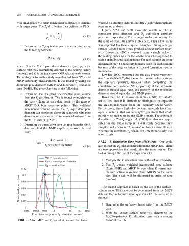
2. Determine the weighted incremental pore volume diameter should equal the total NMR porosity.
from the T distribution. This is found by multiplying However, the T relaxation times (PSD) for shales
2
2
the pore volume at each data point by the ratio of are so low that it is difficult to distinguish or separate
MICP/NMR bins (pressure points). This weighted the clay‐bound water from the capillary‐bound water.
incremental volume versus the T equivalent pore Furthermore, these high clay content materials have ker­
2
diameter can be plotted along the same axis with pore ogen, a material that contains hydrogen atoms that could
diameter versus normalized incremental volume from possibly be picked up by the NMR signals. The approach
the MICP data (Fig. 5.26). described by Zhi‐Qiang et al. (2005) is also not appli­
3. Determine the cumulative pore volume from the NMR cable for the shale samples in our study because their
data and find the NMR capillary pressure derived samples had dominant T relaxation times above 10 m/s,
2
from: whereas the dominant T relaxation time in our study was
2
about 1 m/s.
4 cos b
P NMR 5.7.2.2 T Relaxation Time from MICP Data One could
2
T eqv porediameter (5.14) also extract the T relaxation time from the MICP data. There
2
2
are two approaches that would give the same results. The
first is through the use of the Equation 5.13.
MICP pore diameter 1. Multiply the T relaxation time with surface relaxivity.
T 2 equivalent pore diameter 2
T 2 relaxation time 2. Plot T versus weighted incremental pore volume
2
0.12 (from NMR) and MICP Pc equivalent T versus nor­
2
malized intrusion volume (from MICP) on the same
0.1
plot. The x‐axis will be illustrated in terms of time
Normalized pore volume 0.08 volume ratio. This ratio can be determined from the MICP
(µm/ms).
The second approach is based on the use of the surface–
0.06
data and then substituted into Equation 5.12. The steps are as
0.04
follows:
0.02
1. Determine the surface–volume ratio from the MICP
0 data.
0.0001 0.001 0.01 0.1 1 10 100 1000 2. With the known surface relaxivity, determine the
Pore diameter ( m) or T relaxation time (ms)
2
MICP‐equivalent T relaxation time with a scaling
2
FIGurE 5.26 MICP and T equivalent pore size distribution. factor of c = 3.6.
2