Page 271 - Fundamentals of Gas Shale Reservoirs

GAS FLOW IN A NETWORK OF PORES IN SHALE 251
surface roughness leads to an increase in residence time of 1
molecules in porous media and a decrease in Knudsen dif- 0.9 1: APF (Darabi et al., 2012)
fusivity. D is a quantitative measure of surface roughness 2: Klinkenberg (1941)
3: Civan (2010)
f
that varies between 2 and 3, representing a smooth surface 0.8 4: Darcy (1856) 1
and a space‐filling surface, respectively (Coppens and 0.7 5: Knudsen (Javadpour, 2009)
Dammers, 2006). 2
Civan (2010) permeability model is based on the Beskok 0.6 3
and Karniadakis (1999) approach. The model assumes that Q g /Q g,max 0.5 4
permeability is a function of the intrinsic permeability, the
Knudsen number (K ), the rarefication coefficient α , and the 0.4 5
2
n
slip coefficient b, 0.3
0.2
4 K
k k 1 K 1 n . (11.12) 0.1
n
2
1 bK n
0
0 0.2 0.4 0.6 0.8 1
The dimensionless rarefication coefficient α is given by, t/t max
2
1
1: APF (Darabi et al., 2012)
K B 0.9 2: Klinkenberg (1941)
n . (11.13)
2 0 B 3: Civan (2010) 1
AK
n 0.8 4: Darcy (1856)
5: Knudsen (Javadpour, 2009)
0.7
The lower limit of α (α = 0) corresponds to the slip flow 2
2
2
regime and the upper limit α corresponds to the asymptotic 0.6 3
0
limit of α when K → ∞, which corresponds to the free Q g /Q g,max 0.5 4
n
2
molecular flow. A and B serve as the fitting parameters that 5
may be appropriately adjusted based on the dominant flow 0.4
regime in the shale porous media. Civan (2010) reports the 0.3
adjusted parameter values, A = 0.178, B = 0.4348, and
α = 0.1358 for modeling gas flow in a tight sand example. 0.2
0
Civan (2010) assumes b = −1 based on the Beskok and 0.1
Karniadakis (1999) estimate and subsequently estimates the
Knudsen number as (Jones and Owens, 1980), 0 0 0.2 0.4 0.6 0.8 1
t/t max
K 12 639 k 13 . (11.14)
/
.
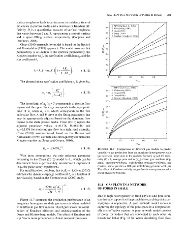
n FIGURE 11.7 Comparison of different gas models to predict
cumulative gas production from an imaginary homogeneous shale
With these assumptions, the only unknown parameter gas reservoir. Input data to the models; Porosity (φ) = 0.05, tortu-
remaining in the Civan (2010) model is k , which can be osity (T) = 5, average pore radius (r ) = 5 nm, gas: methane (top)
avg
∞
determined from a permeability measurement experiment initial pressure = 5000 psi, well‐flowing pressure = 1000 psi, and
(e.g., the pulse‐decay experiment). (bottom) initial pressure = 1000 psi, well‐flowing pressure = 100 psi.
For small Knudsen numbers, that is, K << 1, Civan (2010) The effect of Knudsen and slip on gas flow is more pronounced at
n
estimates the dynamic slippage coefficient b as a function of lower pressures (bottom).
k
gas viscosity, based on the Florence et al. (2007) study,
05 . 11.4 GAS FLOW IN A NETWORK
2790 K
b . (11.15) OF PORES IN SHALE
k
M
Due to high heterogeneity in fluid physics and pore struc-
Figure 11.7 compares the production performance of an ture in shale, a pore level approach in researching shale pet-
imaginary homogeneous shale gas reservoir when modeled rophysics is imperative. A pore network model serves in
with different gas‐flow models. This figure shows the contri- capturing the topology of the pore space in a computation-
bution of Knudsen diffusion and underestimation of the ally cost‐effective manner. A pore network model consists
Darcy and Klinkenberg models. The effect of Knudsen and of pores (or nodes) that are connected to each other via
slip flow is more pronounced at lower reservoir pressures. throats (or links) (Fig. 11.8). When simulating fluid flow,