Page 448 - Fundamentals of Water Treatment Unit Processes : Physical, Chemical, and Biological

Slow Sand Filtration 403

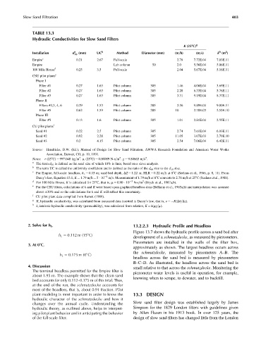
TABLE 13.3
Hydraulic Conductivities for Slow Sand Filters
K (258C) g
h
2
Installation d a 10 (mm) UC b Method Diameter (mm) (m=h) (m=s) k (m )
Empire c 0.21 2.67 Full-scale 2.78 7.72E.04 7.03E.11
Empire Lab column 50 2.0 5.56E.04 5.06E.11
100 Mile House d 0.25 3.5 Full-scale 2.04 5.67E.04 5.16E.11
CSU pilot plants e
Phase I
Filter #1 0.27 1.63 Pilot column 305 1.46 4.06E.04 3.69E.11
Filter #2 0.27 1.63 Pilot column 305 2.28 6.33E.04 5.76E.11
Filter #3 0.27 1.63 Pilot column 305 3.31 9.19E.04 8.37E.11
Phase II
Filters #2,3, 4, 6 0.29 1.53 Pilot column 305 3.56 9.89E.04 9.00E.11
Filter #5 0.62 1.59 Pilot column 305 10 2.78E.03 2.53E.10
Phase III
Filter #5 0.13 1.6 Pilot column 305 1.01 2.81E.04 2.55E.11
CU pilot plants f
Sand #1 0.22 2.5 Pilot column 305 2.74 7.61E.04 6.93E.11
Sand #2 0.92 2.28 Pilot column 305 11.05 3.07E.03 2.79E.10
Sand #3 0.2 4.15 Pilot column 305 2.54 7.06E.04 6.42E.11
Source: Hendricks, D.W. (Ed.), Manual of Design for Slow Sand Filtration, AWWA Research Foundation and American Water Works
Association, Denver, CO, p. 19, 1991.
2
2
3
Notes: r (258C) ¼ 997.048 kg=m . m (258C) ¼ 0.00089 N-s=m . g ¼ 9.80665 m=s .
a
The term d 10 is defined as the sand size of which 10% is finer, based on a sieve analysis.
b
The term UC is called the uniformity coefficient and is defined as the ratio of the d 60 size to the d 10 size.
c
For Empire, full-scale: headloss, h L ¼ 0.15 m; sand bed depth, DZ ¼ 1.22 m; HLR ¼ 0.22 m=hat88C (Seelaus et al., 1986, p. 8, 11). From
Darcy’s law, Equation 13.1, K ¼ 1.79 m=h ¼ 5 10 4 m=s. Measurement of 1.79 m=hat88C converts to 2.78 m=hat258C (Seelaus et al., 1988).
d 3 2
For 100 Mile House, K is calculated for 258C, that is, m ¼ 0.90 10 N-s=m (Bryck et al., 1987a,b).
e
For the CSU filters, calculations of k and K were based upon graphical headloss data (Bellamy et al., 1985a,b) and interpolation was accurate
about 30% and so the calculations for k and K will reflect this uncertainty.
f
CU pilot plant data compiled from Barrett (1989).
g
K, hydraulic conductivity, was calculated from measured data inserted in Darcy’s law, that is, v ¼ K(Dh=Dz).
h
k, intrinsic hydraulic conductivity (permeability), was calculated from relation, K ¼ k(rg=m).
2. Solve for h L , 13.2.2.3 Hydraulic Profile and Headloss
Figure 13.7 shows the hydraulic profile across a sand bed after
h L ¼ 0:112 m (15 C)

development of a schmutzdecke, as measured by piezometers.
Piezometers are installed in the walls of the filter box,
3. At 08C,
approximately as shown. The largest headloss occurs across
the schmutzdecke, measured by piezometers A–B. The
h L ¼ 0:175 m (0 C)

headloss across the sand bed is measured by piezometers
B–C–D. As illustrated, the headloss across the sand bed is
4. Discussion small relative to that across the schmutzdecke. Monitoring the
The terminal headloss permitted for the Empire filter is piezometer water levels is useful in operation, for example,
about 1.95 m. The example shows that the clean sand
bed accounts for only 0.112–0.175 m of this total. Thus, knowing when to scrape, to dewater, and to backfill.
at the end of the run, the schmutzdecke accounts for
most of the headloss, that is, about 0.91 fraction. Pilot
plant modeling is most important in order to know the 13.3 DESIGN
hydraulic character of the schmutzdecke and how it
changes over the annual cycle. Understanding the Slow sand filter design was established largely by James
hydraulic theory, as outlined above, helps in interpret- Simpson for the 1829 London filters with guidelines given
ing pilot plant behavior and in anticipating the behavior by Allen Hazen in his 1913 book. In over 125 years, the
of the full-scale filter. design of slow sand filters has changed little from the London