Page 134 - Geochemical Anomaly and Mineral Prospectivity Mapping in GIS

Catchment Basin Analysis of Stream Sediment Anomalies 133

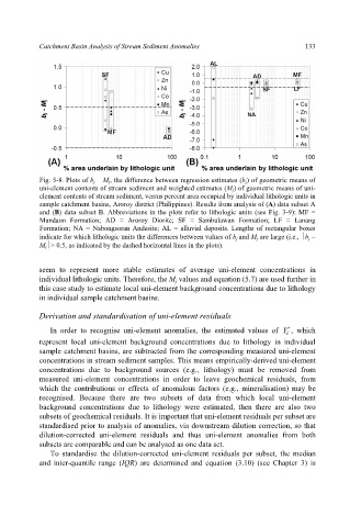
Fig. 5-8. Plots of b j – M j , the difference between regression estimates (b j ) of geometric means of
uni-element contents of stream sediment and weighted estimates (M j ) of geometric means of uni-
element contents of stream sediment, versus percent area occupied by individual lithologic units in
sample catchment basins, Aroroy district (Philippines). Results from analysis of (A) data subset A
and (B) data subset B. Abbreviations in the plots refer to lithologic units (see Fig. 3-9): MF =
Mandaon Formation; AD = Aroroy Diorite; SF = Sambulawan Formation; LF = Lanang
Formation; NA = Nabongsoran Andesite; AL = alluvial deposits. Lengths of rectangular boxes
indicate for which lithologic units the differences between values of b j and M j are large (i.e., ⏐b j –
M j ⏐> 0.5, as indicated by the dashed horizontal lines in the plots).

seem to represent more stable estimates of average uni-element concentrations in
individual lithologic units. Therefore, the M j values and equation (5.7) are used further in
this case study to estimate local uni-element background concentrations due to lithology
in individual sample catchment basins.

Derivation and standardisation of uni-element residuals
In order to recognise uni-element anomalies, the estimated values of Y′ , which
i
represent local uni-element background concentrations due to lithology in individual
sample catchment basins, are subtracted from the corresponding measured uni-element
concentrations in stream sediment samples. This means empirically-derived uni-element
concentrations due to background sources (e.g., lithology) must be removed from
measured uni-element concentrations in order to leave geochemical residuals, from
which the contributions or effects of anomalous factors (e.g., mineralisation) may be
recognised. Because there are two subsets of data from which local uni-element
background concentrations due to lithology were estimated, then there are also two
subsets of geochemical residuals. It is important that uni-element residuals per subset are
standardised prior to analysis of anomalies, via downstream dilution correction, so that
dilution-corrected uni-element residuals and thus uni-element anomalies from both
subsets are comparable and can be analysed as one data set.
To standardise the dilution-corrected uni-element residuals per subset, the median
and inter-quantile range (IQR) are determined and equation (3.10) (see Chapter 3) is