Page 99 - Geochemical Anomaly and Mineral Prospectivity Mapping in GIS

98 Chapter 4

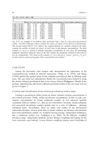
Fig. 4-10. An example of an attribute table associated with a map of a discretised geochemical
surface. The first (leftmost) column contains the names of classes of uni-element concentrations.
The second column (NPIX_CL), which is the original attribute (or variable) column in the table,
contains the number of pixels (or boxes) of each class of uni-element concentrations. The third
column (cl_min) is created to indicate minimum concentration of each class. By performing
arithmetic operations using the values in the first column, the remaining columns are derived (see
text for explanations). The values in the columns cl_min and npix_equal_above_cl_min
are then used to create log-log plots of the concentration-area relation.

CASE STUDY
Among the previously cited workers who demonstrated the application of the
concentration-area method in mineral exploration, Cheng et al. (1996) and Cheng
(1999b) applied the method using stream sediment geochemical data in different study
areas. The case study here demonstrates further the concentration-area method by using
the stream sediment geochemical data in the Aroroy district (Philippines). Details of the
geology, mineralisation and stream sediment geochemical data of the case study area are
given in Chapter 3.

Creation and classification of uni-element geochemical surface maps
Creating a geochemical surface based on stream sediment element concentrations is
not a trivial procedure. Firstly, unlike uni-element concentrations in soils or rocks, uni-
element concentrations in stream sediments actually do not represent spatially
continuous fields or variables (i.e., they are not everywhere). Secondly, stream sediments
and associated uni-element contents pertain only to a zone of influence – drainage
catchment basin. Nevertheless, there are many case studies in the geochemical
exploration literature wherein point data of stream sediment uni-element concentrations
have been transformed, usually via ‘weighted moving average’ interpolation techniques,
into a continuous surface (e.g., Ludington et al., 2006). Of the different ‘weighted
moving average’ interpolation methods, inverse distance weighting and kriging are the
most commonly used methods. Inverse distance weighting requires some knowledge of