Page 210 - Handbook Of Integral Equations

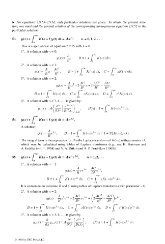
For equations 2.9.53–2.9.62, only particular solutions are given. To obtain the general solu-
tion, one must add the general solution of the corresponding homogeneous equation 2.9.52 to the
particular solution.

∞

n
53. y(x)+ K(x – t)y(t) dt = Ax , n =0, 1, 2, ...
x
This is a special case of equation 2.9.55 with λ =0.
1 . A solution with n =0:
◦
A ∞
y(x)= , B =1 + K(–z) dz.
B 0
◦
2 . A solution with n =1:
A AC ∞ ∞
y(x)= x – , B =1 + K(–z) dz, C = zK(–z) dz.
B B 2
0 0
3 . A solution with n =2:
◦
A 2 AC AC 2 AD
y 2 (x)= x – 2 x +2 – ,
B B 2 B 3 B 2
∞ ∞ ∞

2
B =1 + K(–z) dz, C = zK(–z) dz, D = z K(–z) dz.
0 0 0
◦
4 . A solution with n =3, 4, ... is given by:
∞
∂ n e λx
λz
y n (x)= A , B(λ)=1 + K(–z)e dz.
∂λ n B(λ)
λ=0 0
∞

54. y(x)+ K(x – t)y(t) dt = Ae λx .
x
A solution:
A λx ∞ λz
y(x)= e , B =1 + K(–z)e dz =1 + L{K(–z), –λ}.
B 0
The integral term in the expression for B is the Laplace transform of K(–z) with parameter –λ,
which may be calculated using tables of Laplace transforms (e.g., see H. Bateman and
A. Erd´ elyi (vol. 1, 1954) and V. A. Ditkin and A. P. Prudnikov (1965)).
∞

n λx
55. y(x)+ K(x – t)y(t) dt = Ax e , n =1, 2, ...
x
1 . A solution with n =1:
◦
A λx AC λx
y 1 (x)= xe – e ,
B B 2
∞ ∞

B =1 + K(–z)e λz dz, C = zK(–z)e λz dz.
0 0
It is convenient to calculate B and C using tables of Laplace transforms (with parameter –λ).
2 . A solution with n =2:
◦
A 2 λx AC λx AC 2 AD λx
y 2 (x)= x e – 2 xe + 2 – e ,
B B 2 B 3 B 2
∞ ∞ ∞

2
B =1 + K(–z)e λz dz, C = zK(–z)e λz dz, D = z K(–z)e λz dz.
0 0 0
3 . A solution with n =3, 4, ... is given by
◦
∂ ∂ n e λx ∞ λz
y n (x)= y n–1 (x)= A , B(λ)=1 + K(–z)e dz.
∂λ ∂λ n B(λ) 0
© 1998 by CRC Press LLC

© 1998 by CRC Press LLC
Page 189