Page 222 - Hydrogeology Principles and Practice

HYDC06 12/5/05 5:33 PM Page 205

Groundwater quality and contaminant hydrogeology 205

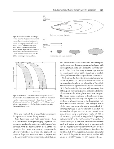
Fig. 6.4 Dispersion within an isotropic
porous material of (a) a continuous point
source of pollution at various times, t,
and (b) an instantaneous (single event)
point source of pollution. Spreading
of the pollution plumes results from
hydrodynamic dispersion and acts to dilute
the contaminant concentrations, while
advection transports the plumes in the
field of uniform groundwater flow.

The variance tensor can be resolved into three prin-
cipal components that are approximately aligned with
the longitudinal, transverse horizontal and transverse
vertical directions. Assuming a constant groundwa-
ter velocity, dispersivity can be calculated as one half
of the gradient of the linear spatial trend in variance.
To illustrate the dispersive transport of groundwa-
ter solutes, Hess et al. (2002) conducted a tracer test in
the unconfined sand and gravel aquifer of Cape Cod,
Massachusetts using the conservative tracer bromide
−
(Br ). As shown in Fig. 6.6a, and with increasing time
of transport, physical dispersion of the injected mass
of tracer causes the solute plume to become elongate.
Fig. 6.5 Positions of a contaminant front transported by one- The tracer plume continued to lengthen as it trav-
dimensional molecular diffusion at times of 100 years and 10,000
elled down-gradient through the aquifer and should
years for a source concentration, C = C , at time, t > 0, and a
0 conform to a linear increase in the longitudinal vari-
2 −1
diffusion coefficient, D*, of 10 −10 and 10 −11 m s . The curves of
ance with distance travelled. The synoptic results
relative concentration are calculated using equation 6.5. After
Freeze and Cherry (1979). of the tracer test showed that the longitudinal Br −
variance increased at a slow rate early in the test but
increased at a larger rate after about 70 m of trans-
100 m, as a result of the physical heterogeneities in port. A linear trend fit to the later results (69–109 m
the aquifer encountered during transport. of transport) produced a longitudinal dispersivity
−
Both laboratory and field experiments show estimate for Br of 2.2 m (Fig. 6.6b). The number of
that contaminant mass spreading by dispersion in a observations (n = 4) on which this estimate is based is
porous material conforms to a normal (Gaussian) dis- small and scatter around the trend is apparent such
tribution, with the position of the mean of the con- that the dispersive process may not yet have reached
centration distribution representing transport at the a constant asymptotic value of longitudinal dispersiv-
advective velocity of the water. The degree of con- ity (Hess et al. 2002). In general, transverse horizontal
taminant dispersion about the mean is proportional and vertical dispersivities were much smaller with
−2
−4
2
to the variance (σ ) of the concentration distribution. values of 1.4 × 10 m and 5 × 10 m, respectively.