Page 223 - Hydrogeology Principles and Practice

HYDC06 12/5/05 5:33 PM Page 206

206 Chapter Six

Combining the mathematical description of
mechanical dispersion with the molecular diffusion
coefficient gives an expression for the hydrodynamic
dispersion coefficient, D, as follows:

D = α V + D*
l l l
eq. 6.6
D = α V + D*
t t t
where the subscripts and indicate the longitudinal
l t
and transverse directions, respectively.
The relative effects of mechanical dispersion
and molecular diffusion can be demonstrated from
the results of a controlled column experiment. The
breakthrough curve for a continuous supply of tracer
fed into a column packed with granular material is
shown in Fig. 6.7. At low tracer velocity, molecular
diffusion is the important contributor to hydrodyn-
amic dispersion, although with little effect in spread-
ing the tracer front. At high velocity, mechanical
dispersion dominates and the breakthrough curve
adopts a characteristic S-shape with some of the
tracer moving ahead of the advancing front and
some lagging behind, as controlled by the tortuosity
of the flowpaths. The midpoint of the breakthrough
curve occurs for a relative concentration, C/C , equal
0
to one-half. This point of half-concentration repres-
ents the advective behaviour of the solute transport
(shown by the vertical dashed line in Fig. 6.7) as if the
tracer were moving by a plug-flow-type mechanism.

One-dimensional solute transport equation
Following from the above description of solute
transport processes, the one-dimensional form of the
solute transport equation describing the time-varying
change in concentration of non-reactive dissolved
contaminants in saturated, homogeneous, isotropic
material under steady-state, uniform flow conditions

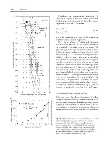
Fig. 6.6 (left) Results of a tracer experiment in the Cape Cod sand
and gravel aquifer showing: (a) the distributions of relative
−
concentrations (C/C ) of Br observed 13 and 83 days after
0
injection (dashed where inferred); (b) calculated longitudinal
−
variances of the Br tracer plume for each synoptic sampling
round. Also shown in (a) are locations of multilevel samplers
available for groundwater sampling (solid circles) and tracer
injection (solid squares). After Hess et al. (2002).