Page 226 - Hydrogeology Principles and Practice

HYDC06 12/5/05 5:33 PM Page 209

BO X
Macrodispersion caused by layered heterogeneity
6.2

The effect of macrodispersion in a layered aquifer system on the laden flow in this layer contributes 23% (0.4/1.75) of the actual
transport of a reactive contaminant can be demonstrated by com- flow through the aquifer. Thus, the relative concentration of the
bining Darcy’s law (eq. 2.5) and the retardation equation (eq. 6.13) chemical in the well at this time, which is found from the concentra-
to derive the shape of the relative concentration breakthrough tion in the well water, C, as a fraction of the original source con-
3
curve. For the example of layered heterogeneity shown in Fig. 1, and centration, C , also equals 0.23. After 25 × 10 days, the flow of
0
−1
3
for a well positioned at 1000 m from the pollution source and contaminated water at the well increases to 1.4 m day (0.4 + 1),
−1
3
pumping at 1.75 m day , then assuming saturated flow under a or 80% of flow from the aquifer. The calculation is continued until
3
hydraulic gradient of 0.01 in each layer, the relative breakthrough 303 × 10 days when the relative concentration C/C of the well
0
concentration in each layer can be calculated as shown in Table 1. water equals 1.
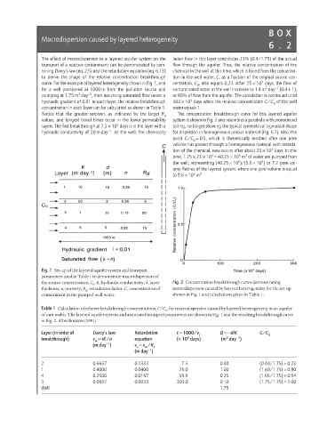
Notice that the greater sorption, as indicated by the larger R The concentration breakthrough curve for this layered aquifer
d
values, and longest travel times occur in the lower permeability system is shown in Fig. 2 and resembles a parabola with pronounced
3
layers. The first breakthrough at 7.5 × 10 days is in the layer with a tailing, no longer showing the typical symmetrical sigmoidal shape
−1
hydraulic conductivity of 20 m day . At the well, the chemically for dispersion in homogeneous porous material (Fig. 6.7). Also, the
point C/C = 0.5, which is theoretically reached after one pore
0
volume has passed through a homogeneous material with retarda-
3
tion of the chemical, now occurs after about 23 × 10 days. In this
3
3
3
time, 1.75 × 23 × 10 = 40.25 × 10 m of water are pumped from
3
3
the well, representing (40.25 × 10 )/(5.6 × 10 ) or 7.2 pore vol-
ume flushes of the layered system, where one pore volume is equal
3
3
to 5.6 × 10 m .

Fig. 1 Set-up of the layered aquifer system and transport
parameters used in Table 1 to demonstrate macrodispersion of
the source concentration, C . K, hydraulic conductivity; d, layer Fig. 2 Concentration breakthrough curve demonstrating
0
thickness; n, porosity; R , retardation factor; C, concentration of macrodispersion caused by layered heterogeneity for the set-up
d
contaminant in the pumped well water. shown in Fig. 1 and calculations given in Table 1.
Table 1 Calculation of relative breakthrough concentrations, C/C , for macrodispersion caused by layered heterogeneity in an aquifer
o
of unit width. The layered aquifer system and associated transport parameters are shown in Fig. 1 and the resulting breakthrough curve
in Fig. 2. After Bouwer (1991).
Layer (in order of Darcy’s law: Retardation t = 1000/v c Q =−diK C/C o
−1
3
3
breakthrough) v = iK/n equation (× 10 days) (m day )
w
−1
(m day ) v = v /R t
w
c
−1
(m day )
2 0.6667 0.1333 7.5 0.40 (0.40/1.75) = 0.23
1 0.4000 0.0400 25.0 1.00 (1.40/1.75) = 0.80
4 0.2500 0.0167 59.9 0.25 (1.65/1.75) = 0.94
3 0.0667 0.0033 303.0 0.10 (1.75/1.75) = 1.00
Well 1.75