Page 224 - Hydrogeology Principles and Practice

HYDC06 12/5/05 5:33 PM Page 207

Groundwater quality and contaminant hydrogeology 207

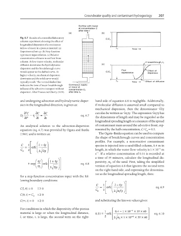
Fig. 6.7 Results of a controlled laboratory
column experiment showing the effect of
longitudinal dispersion of a continuous
inflow of tracer in a porous material. (a)
Experimental set-up. (b) Step-function
type tracer input relation. (c) Relative
concentration of tracer in outflow from
column. At low tracer velocity, molecular
diffusion dominates the hydrodynamic
dispersion and the breakthrough curve
would appear as the dashed curve. At
higher velocity, mechanical dispersion
dominates and the solid curve would
typically result. The vertical dashed line
indicates the time of tracer breakthrough
influenced by advective transport without
dispersion. After Freeze and Cherry (1979).

and undergoing advection and hydrodynamic disper- hand side of equation 6.8 is negligible. Additionally,
sion in the longitudinal direction, is given as: if molecular diffusion is assumed small compared to
mechanical dispersion, then the denominator √D t l
∂ 2 C ∂ C ∂ C can also be written as √α V t. The expression √α V t has
=
−
D l V l eq. 6.7 l l l l
l ∂ 2 l ∂ t ∂ the dimensions of length and may be regarded as the
longitudinal spreading length or a measure of the spread
An analytical solution to the advection-dispersion of contaminant mass around the advective front, rep-
equation (eq. 6.7) was provided by Ogata and Banks resented by the half-concentration, C/C = 0.5.
0
(1961) and is written as: The Ogata–Banks equation can be used to compute
the shape of breakthrough curves and concentration
⎡ ⎛ ⎞ profiles. For example, a non-reactive contaminant
−
C 1 ⎢ l V l t species is injected into a sand-filled column, 0.4 m in
=
erfc ⎜ ⎟
−4
C 0 2 ⎢ ⎜ ⎝ 2 Dt ⎠ ⎟ length, in which the water flow velocity is 1 × 10 m
⎣ l s . If a relative concentration of 0.31 is recorded at
−1
⎛ V l ⎞ ⎛ l + V t ⎞⎤ ⎥ a time of 35 minutes, calculate the longitudinal dis-
persivity, α , of the sand. First, taking the simplified
+ exp ⎜ l ⎟ erfc ⎜ ⎜ l ⎟ eq. 6.8 l
⎝ D l ⎠ ⎝ 2 Dt ⎟ ⎥ version of equation 6.8 that ignores the second term
⎠
l ⎦ on the right-hand side, and expressing the denomina-
tor as the longitudinal spreading length, then:
for a step-function concentration input with the fol-
lowing boundary conditions:
⎡ ⎛ ⎞⎤
−
C = 1 ⎢ l V l t ⎥
C(l, 0) = 0 l ≥ 0 2 ⎢ erfc ⎜ ⎜ ⎟ ⎟ ⎥ eq. 6.9
C 0 ⎝ 2 α V t ⎠
⎣ ll ⎦
C(0, t) = C t ≥ 0
0
C(∞, t) = 0 t ≥ 0 and substituting the known values gives:
For conditions in which the dispersivity of the porous ⎡ ⎤
1 10 ×

1 04 −× 4 − 35 × 60
.
material is large or when the longitudinal distance, 031. = erfc ⎢ ⎥ eq. 6.10
1 10 ×
l, or time, t, is large, the second term on the right- 2 ⎢ ⎣ 2 α ×× 4 − 35 × 60 ⎥ ⎦

l