Page 127 - Introduction to Mineral Exploration

110 M.K.G. WHATELEY

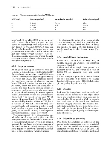
TABLE 6.3 False colors assigned to Landsat MSS bands.

MSS band Wavelength (µµ µµ µm) Natural color recorded False color assigned
4 0.5–0.6 Green Blue
5 0.6–0.7 Red Green
6 0.7–0.8 IR Red
7 0.8–1.1 IR Red

from black (0) to white (255), giving us a gray A photographic print of a geometrically
scale. Commonly 6 bits per pixel (64 gray corrected image (Fig. 6.5) is a parallelogram.
levels) are used for MSS and 8 bits per pixel (256 The earth rotates during the time it takes
gray levels) for TM and ASTER. A pixel can the satellite to scan a 185 km length of its
therefore be located in the image by an x and swath, resulting in the skewed image (Fig.
y co-ordinate, while the z value defines the 6.11f).
gray-scale value between 0 and 255. Pixel size
determines spatial resolution whilst the radi-
ance quantization affects radiometric resolu- 6.2.4 Availability of Landsat data
tion (Schowengerdt 1983). 1 Landsat CCTs or CDs of MSS, TM, or
ASTER imagery are available for computer
processing (Box 6.1).
6.2.3 Image parameters
2 Black and white, single band prints in a
An image is built up of a series of rows and standard 23 cm × 23 cm format at a scale of
columns of pixels. Rows of pixels multiplied by 1:1000,000 are available from the above
the number of columns in a typical MSS image sources.
(3240 × 2340 respectively) gives approximately 3 Color composite prints in a similar format
7M pixels per image. The improved resolu- are also available. It is possible to enlarge
tion and larger number of channels scanned Landsat MSS images up to 1:100,000, before the
by the TM results in nine times as many pixels picture quality degrades severely.
per scene, hence the need for computers to
analyze the data. Remote sensing images are
commonly multispectral, e.g. the same scene 6.2.5 Mosaics
is imaged simultaneously in several spectral Each satellite image has a uniform scale and
bands. Landsat MSS records four spectral bands relative lack of distortion at the edges. Black
(Table 6.3), TM records seven, and ASTER and white or color prints of each scene can be
records 14 spectral bands. Visible blue light is cut and spliced into mosaics. With the repetit-
not recorded by Landsat MSS or ASTER, but it ive cover most of the world has cloud-free
is recorded in TM band 1. By combining three Landsat imagery available. The biggest diffi-
spectral bands and assigning a color to each culty is in matching the gray tone during print-
band (so that the gray scale becomes a red, ing, and the images from different seasons.
green, or blue scale instead), a multispectral Scenes can be merged digitally to alleviate gray
false color composite image is produced. tone differences.
The image intensity level histogram is a use-
ful indicator of image quality (Fig. 6.4). The
histogram describes the statistical distribution 6.2.6 Digital image processing
of intensity levels or gray levels in an image in Data from the satellites are collected at the
terms of the number of pixels (or percentage of ground station on magnetic tape, i.e. in a digital
the total number of pixels) having each gray form. Data are loaded into image processing
level. Figure 6.4 shows the general character- computer systems from CCTs or CDs. The
istics of histograms for a variety of images. main functions of these systems in a geological