Page 156 - Introduction to Mineral Exploration

7: GEOPHYSICAL METHODS 139

Schlumberger: L/h
k = 1.0 0.9 0.8

ρ
ρ 2 – ρ 1 ρ
k = ρ 0.7
ρ 2 + ρ 1 ρ
Schlumberger
“cross” 0.6
Wenner 0.5
“cross”
0.4
0.3
0.2
ρ α α ρ 0.1
ρ α / ρ 1 = 1
ρ α /ρ 1 ρρ α 0.0
−0.1
−0.2
−0.3
−0.4
“Cross” for Wenner −0.5
or Schlumberger
field curve plotted −0.6
using total array L/h = 1 (Schlumberger) a/h = 1 (Wenner)
length (2L) as −0.7
ordinate k = −1.0 L/h = 10 a/h = 10

−0.9
Wenner: a/h (= 2L/3h) −0.8
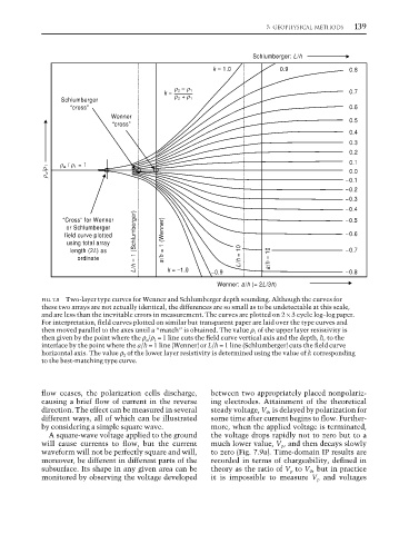
FIG. 7.8 Two-layer type curves for Wenner and Schlumberger depth sounding. Although the curves for
these two arrays are not actually identical, the differences are so small as to be undetectable at this scale,
and are less than the inevitable errors in measurement. The curves are plotted on 2 × 3 cycle log–log paper.
For interpretation, field curves plotted on similar but transparent paper are laid over the type curves and
then moved parallel to the axes until a “match” is obtained. The value ρ 1 of the upper layer resistivity is
then given by the point where the ρ a /ρ 1 = 1 line cuts the field curve vertical axis and the depth, h, to the
interface by the point where the a/h = 1 line (Wenner) or L/h = 1 line (Schlumberger) cuts the field curve
horizontal axis. The value ρ 2 of the lower layer resistivity is determined using the value of k corresponding
to the best-matching type curve.

flow ceases, the polarization cells discharge, between two appropriately placed nonpolariz-
causing a brief flow of current in the reverse ing electrodes. Attainment of the theoretical
direction. The effect can be measured in several steady voltage, V 0 , is delayed by polarization for
different ways, all of which can be illustrated some time after current begins to flow. Further-
by considering a simple square wave. more, when the applied voltage is terminated,
A square-wave voltage applied to the ground the voltage drops rapidly not to zero but to a
will cause currents to flow, but the current much lower value, V p , and then decays slowly
waveform will not be perfectly square and will, to zero (Fig. 7.9a). Time-domain IP results are
moreover, be different in different parts of the recorded in terms of chargeability, defined in
subsurface. Its shape in any given area can be theory as the ratio of V p to V 0 , but in practice
monitored by observing the voltage developed it is impossible to measure V p and voltages