Page 74 - Lindens Handbook of Batteries

ELECTROCHEMICAL PRINCIPLES AND REACTIONS 2.31

Current

E 1
E o

Time
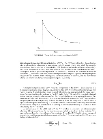
FIGURE 2.38 Typical single step constant potential pulse for PITT.

Potentiostatic Intermittent Titration Technique (PITT). The PITT method involves the application
of a small amplitude voltage step to an electrode, typically around 10 mV, after which the current is
recorded as a function of time, as shown in Fig. 2.38. Starting at an initial equilibrium voltage of E ,
o
the current decays to zero or very near (negligible) to zero, reaching a new equilibrium potential E .
1
Subsequent potential pulses are imposed on the electrode to determine the incremental charge in
coulombs, Q, associated with each pulse covering the whole range of capacity defining the phase
diagram for the material under investigation. The total current I is recorded, and the incremental
charge (or differential charge) for each potential pulse is given by

Q = ∫ t Idt (2.60)
0
Plotting the rest potential (the OCV) versus the composition of the electrode material results in a
figure representing the phase diagram, i.e., similar to Fig. 2.37. Plots of the differential charge Q/E
versus potential E results in sharp peaks precisely identifying the peak potentials for phase transi-
36
tions. An example of this plot is shown in Fig. 2.39 for Li CoO . Figure 2.39 is essentially identical
2
x
to that obtained by cyclic voltammetry (Sec. 2.6.1 above), but there are important differences. The
peak potentials for each phase are very sharp compared to what is observed in fast CV sweeps where
the peak potentials are not precisely defined. By slowing down the sweep rate to ~0.001 mV/s, a
37
cyclic voltammogram similar to Fig. 2.39 can be obtained, but because of the very low currents
for such a low sweep rate, determination of capacity is difficult and not nearly as accurate as those
obtained by the PITT method.
34
As demonstrated for the GITT method , the PITT method is also useful for determining the
chemical diffusion coefficient for the insertion or removal of an ion from its host material. Two
approaches are based on the thickness of the electrode, L [see Eq. (2.59)] and the time, t, required
36
to reach the equilibrium potential after each potential pulse. The relations from Ref. 36 are given
in Eqs. (2.61) and (2.62).
/ 
QD 12 1 
2
I() t =   if t << L /D (2.61)
Lπ / 12 t  / 12 