Page 131 - MATLAB an introduction with applications
P. 131

116 ———  MATLAB: An Introduction with Applications


                   semilogx(f,phase,‘Linewidth’,2);
                         %PHASE
                   title(‘\bfPlot of phase of current flow vs frequency’);
                   xlabel(‘\bfFrequency (Hz)’);
                   ylabel(‘\bfPhase (Deg)’);
                   grid on;

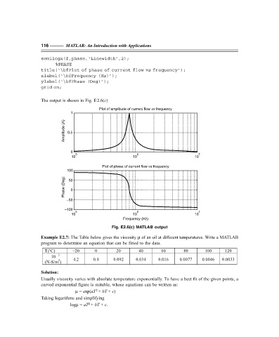
                   The output is shown in Fig. E2.6(c)

                                            Plot of amplitude of current flow vs  frequency
                                1
                             (A)
                             Amplitude  0.5


                                0
                                  5                          6                          7
                                10                         10                         10

                                              Plot of phase of current flow vs  frequency
                              100
                             (Deg)  50
                             Phase  0


                              –50
                             –100
                                  5                          6                          7
                                10                         10                         10
                                                       Frequency (Hz)
                                                  Fig. E2.6(c) MATLAB output

                   Example E2.7: The Table below gives the viscosity µ of an oil at different temperatures. Write a MATLAB
                   program to determine an equation that can be fitted to the data.
                     T(°C)       –20       0        20        40        60       80        100      120

                          –5
                       10

                           2
                     (N-S/m )    4.2      0.4      0.092     0.034    0.016     0.0077    0.0046  0.0033
                   Solution:
                   Usually viscosity varies with absolute temperature exponentially. To have a best fit of the given points, a
                   curved exponential figure is suitable, whose equations can be written as:
                                    µ = exp(aT + bT + c)
                                           2
                   Taking logarithms and simplifying
                                        2
                                logµ = aT + bT + c.


                   F:\Final Book\Sanjay\IIIrd Printout\Dt. 10-03-09
   126   127   128   129   130   131   132   133   134   135   136