Page 132 - MATLAB an introduction with applications

Electrical Circuits ——— 117

here the constants can be obtained from the polyfit function polyfit(T, logµ, 2), then finally µ is obtained
from the exponential relation and ploted as a function of temperature in Kelvin.

MATLAB program for this application is shown below:
TC=–20:20:120;
%TEMPERATURE RANGE IN DEGREE CENTRIGRADE
mu=[4.2 0.4 0.092 0.034 0.016 0.0077 0.0046 0.0033]; %GIVEN VISCOSITIES
TK=TC + 273; % TEMPERATURE IN KELVIN
p=polyfit(TK,log(mu),2) % POLYNOMIAL FITTING WITH LOG(MU) AND TK, SECOND ORDER
Tplot=273+[–20:120];% DEFINING TK AS AN ARRAY

muplot= exp(p(1)* Tplot^2+p(2)* Tplot+p(3));%CORRESPONDING MU ARRAY
semilogy(TK,mu,‘o’,Tplot,muplot,‘–’)%PLOTTING ON SEMI–LOG SCALE
xlabel(‘\bfTemperature K’);
ylabel(‘\bfViscosity in N–S/meter square’);

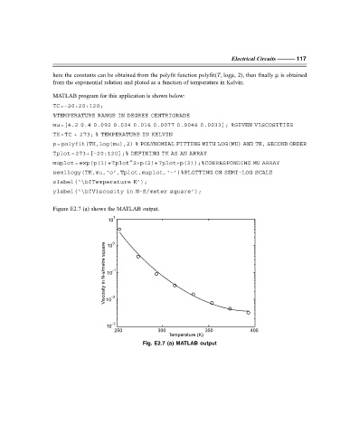
Figure E2.7 (a) shows the MATLAB output.
1
10

square 10 0

N-s/metre 10 –1

in
Viscosity 10 –2

–3
10
250 300 350 400
Temperature (K)
Fig. E2.7 (a) MATLAB output

F:\Final Book\Sanjay\IIIrd Printout\Dt. 10-03-09