Page 135 - MATLAB an introduction with applications

120 ——— MATLAB: An Introduction with Applications

P2.5: The ratio of the magnitude of the voltage in a low-pass RC filter shown in Fig. P2.5 is given by

V 1
RV = 0 =
V i 1( RC+ω ) 2
where ω is the frequency of the input signal.
R
Write a user-defined MATLAB function that calculates the magnitude ratio.
Write a program in script file that uses the lowpass function to generate a plot V i C V o
6
–2
of RV as a function of ω for 10 ≤ ω ≤ 10 rad/s. Run the script file with
R = 1300 Ω, and C = 9 µF.
Fig. P2.5
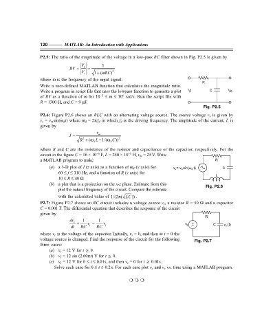
P2.6: Figure P2.6 shows an RLC with an alternating voltage source. The source voltage v s is given by
v s = v m sin(ω d t) where ω d = 2πf d in which f d is the driving frequency. The amplitude of the current, I, is
given by
v
I = m
R +ω d L − 1/(ω d C )) 2
2
(
where R and C are the resistance of the resistor and capacitance of the capacitor, respectively. For the
–3
circuit in the figure C = 16 × 10 F, L = 250 × 10 H, v m = 25V. Write
–6
a MATLAB program to make R
(a) a 3-D plot of I (z axis) as a function of ω d (x axis) for v s = v sin(" d t) C
m
60 ≤ f ≤ 110 Hz, and a function of R (y axis) for
10 ≤ R ≤ 40 Ω L
(b) a plot that is a projection on the x-z plane. Estimate from this
plot the natural frequency of the circuit. Compare the estimate Fig. P2.6
with the calculated value of 1/(2 ( LCπ )) .
P2.7: Figure P2.7 shows an RC circuit includes a voltage source v s , a resistor R = 50 Ω and a capacitor
C = 0.001 F. The differential equation that describes the response of the circuit
given by
R
dv c + 1 v = 1 v
dt RC c RC s v s C v c (t)
where v c is the voltage of the capacitor. Initially, v s = 0, and then at t = 0 the
voltage source is changed. Find the response of the circuit for the following Fig. P2.7
three cases:
(a) v s = 12 V for t ≥ 0.
(b) v s = 12 sin (2.60πt) V for t ≥ 0.
(c) v s = 12 V for 0 ≤ t ≤ 0.01s, and then v s = 0 for t ≥ 0.01s.
Solve each case for 0 ≤ t ≤ 0.2s. For each case plot v s and v c vs. time using a MATLAB program.

❍ ❍ ❍

F:\Final Book\Sanjay\IIIrd Printout\Dt. 10-03-09