Page 48 - MATLAB an introduction with applications

MATLAB Basics ——— 33

Use (i) the plot command
(ii) the hold command
(iii) the line command
(b) Use the functions for plotting x-y data for plotting the following functions:
(i) f(t) = t cost
0 ≤ t ≤ 10π
(ii) x = e t
y = 100 + e 3t
0 ≤ t ≤ 2π
Solution:
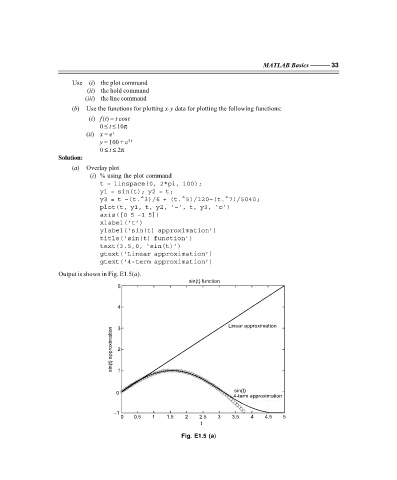
(a) Overlay plot
(i) % using the plot command
t = linspace(0, 2*pi, 100);
y1 = sin(t); y2 = t;
y3 = t –(t.^3)/6 + (t.^5)/120–(t.^7)/5040;
plot(t, y1, t, y2, ‘–’, t, y3, ‘o’)
axis([0 5 –1 5])
xlabel(‘t’)
ylabel(‘sin(t) approximation’)
title(‘sin(t) function’)
text(3.5,0, ‘sin(t)’)
gtext(‘Linear approximation’)
gtext(‘4-term approximation’)
Output is shown in Fig. E1.5(a).
sin(t) function
5

4

Linear approximation
3
approximation 2

)
sin(t 1

sin(t)
0
4-term approximation
–1
0 0.5 1 1.5 2 2.5 3 3.5 4 4.5 5
t

Fig. E1.5 (a)

F:\Final Book\Sanjay\IIIrd Printout\Dt. 10-03-09