Page 49 - MATLAB an introduction with applications

34 ——— MATLAB: An Introduction with Applications

(ii) % using the hold command
x = linspace(0, 2*pi, 100); y1=sin(x);
plot(x,y1)
hold on
y2 = x; plot(x, y2, ‘–’ )
y3 = x–(x.^3)/6 + (x.^5)/120–(t.^7)/5040;
plot(x, y3, ‘o’)
axis([0 5–1 5])
hold off
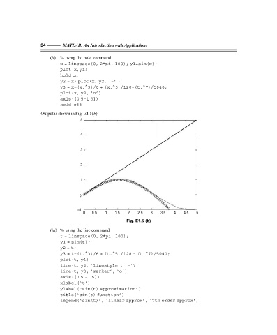
Output is shown in Fig. E1.5(b).
5

4

3

2

1

0

–1
0 0.5 1 1.5 2 2.5 3 3.5 4 4.5 5
Fig. E1.5 (b)
(iii) % using the line command
t = linspace(0, 2*pi, 100);
y1 = sin(t);
y2 = t;
y3 = t–(t.^3)/6 + (t.^5)/120 – (t.^7)/5040;
plot(t, y1)
line(t, y2, ‘linestyle’, ‘–’)
line(t, y3, ‘marker’, ‘o’)
axis([0 5 –1 5])
xlabel(‘t’)
ylabel(‘sin(t) approximation’)
title(‘sin(t) function’)
legend(‘sin(t)’, ‘linear approx’, ‘7th order approx’)

F:\Final Book\Sanjay\IIIrd Printout\Dt. 10-03-09