
Page 50 - MATLAB an introduction with applications
P. 50
MATLAB Basics ——— 35
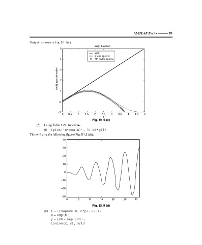
Output is shown in Fig. E1.5(c).
sin(t) function
5
sin(t)
linear approx
4 7th order approx
approximation 3 2
sin(t)
1
0
–1
0 0.5 1 1.5 2 2.5 3 3.5 4 4.5 5
t
Fig. E1.5 (c)
(b) Using Table 1.29, functions
(i) fplot(‘x*cos(x)’, [0 10*pi])
This will give the following figure (Fig. E1.5 (d)).
40
30
20
10
0
–10
–20
–30
0 5 10 15 20 25 30
Fig. E1.5 (d)
(ii) t = linspace(0, 2*pi, 200);
x = exp(t);
y = 100 + exp(3*t);
loglog(x, y), grid
F:\Final Book\Sanjay\IIIrd Printout\Dt. 10-03-09