Page 191 - Mechanics Analysis Composite Materials

176 Mechanics and analysis of composite materials

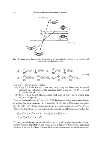
Fig. 4.45. Stress-strain diagrams of a unidirectional ply simulating its behavior in the laminate and
allowing for cracks in the matrix.

A1, = xEf)fit)cEy)$i, A22 = xgg)fig)+xEY),$ji,
n
m
m
n
+
i= 1 j= I i= I j= 1 (4.121)
m n vviEf)@, Ad4 = m n GI,ci)A,,-ii) ,
(j) -(j) -(;)
AI2 = 52EI h, + GI:)&!) +
i=l j= 1 i= 1 j= I
-
where h,-(i) - h,(4/h and = hfi/h.
(a) If ax > 0 in the kth ply, it can work only along the fibers, and we should
calculate the stiffnesses of the degraded layer taking E: = 0, Gf2 = 0, and
vf2 = 0 in Eqs. (4.121).
(b) If U2k < 0 in the kth ply, it cannot work only in shear, so we should take
C& = 0 in Eqs. (4.121).
Thus, we find coefficientsA.!:) (st = 11,12,22,44) corresponding to the second stage
of loading (with one degraded ply). Using Eqs. (4.102) and (4.101) we can determine
EL2',Ef', Gi:), v$), I$? and express the strains in terms of stresses, i.e., $'(o), .$'(o),
y;;)(o). The final strains corresponding to the second stage of loading are calculated as

Exf = &:')(a*) +E:*)(, - 6*), &-; = &;'(a*) +&.f)(, - 6*),
-
71." - y:+;)(.*, + y:;ya - a*).
To study the third stage, we should find QI,~2,212in all the plies, except the kth one,
identify the next degraded ply and repeat step 3 of the procedure which is continued
until the failure of the fibers. The resulting stress-strain curves are multi-segmented