Page 146 -

136 4 Optical Rotor
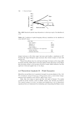
400
300 Slope
Optical torque (pNmm) 100 0 0 20 40 60 Total 80
200

-100
-200 Back side surface Slope angle (deg)
-300

Fig. 4.20. Simulated optical torque dependence on the slope angle of the shuttlecock
rotor

Table 4.2. Conditions of optical trapping efficiency simulation for the shuttlecock
rotor with 45 slopes
◦
rotor size
slope angle a 45 ◦
diameter d 20 µm
thickness t 10 µm
wing width w 5 µm
number of element on the aperture
radial direction 100
circular direction 100

torque increases as the slope angle increases and reaches a maximum at 45 ◦
because the large divergent angle increases the reverse torque at back side
surface III.
Figure 4.21a shows that the total optical torque increases as the wing width
increases and Fig. 4.20b shows that total optical torque decreases as the thick-
ness increases owingto the increase of reverse torque, which indicates that the
optimum thickness equals that of the slope.

4.3Theoretical Analysis II – Fluid Dynamics

Microflow around the rotor is analyzed through the process shown in Fig. 4.22.
The simulation was performed in a 3-D geometry with a commercial compu-
tational fluid dynamics tool (CFX-4, AEA Corp.) [4.11].
First, the rotor shape is input and the cube grid is formed. The initial
conditions of the medium, water at 283 K, density, and viscosity are defined.
The control volume is a cube, in which each domain has a set of discretized
equations that are formulated by evaluatingand integratingthe fluxes across