Page 149 -

4.3 Theoretical Analysis II – Fluid Dynamics 139
(a) 0 60 mm (b) 0 60 mm
0 0

-1 +0.6 m s -1
-1
-0.6 m s
60 5 mm s 60
mm mm
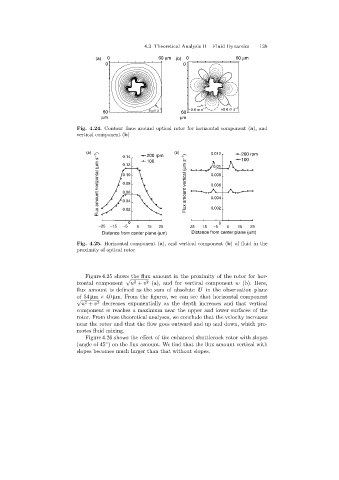
Fig. 4.24. Contour lines around optical rotor for horizontal component (a),and
vertical component (b)

(a) 0.14 200 rpm (b) 0.012 200 rpm
Flux amount horizontal (mm s -1 ) 0.10 Flux amount vertical (mm s -1 ) 0.008
100
100
0.12
0.01
0.08
0.006
0.06
0.004
0.04
0.02
0 0.002 0
-25 -15 -5 5 15 25 -25 -15 -5 5 15 25
Distance from center plane (mm) Distance from center plane (mm)
Fig. 4.25. Horizontal component (a), and vertical component (b)of fluid in the
proximity of optical rotor

Figure 4.25 shows the flux amount in the proximity of the rotor for hor-
√
2
2
izontal component u + v (a), and for vertical component w (b). Here,
flux amount is defined as the sum of absolute U in the observation plane
of 54 µm × 40 µm. From the figures, we can see that horizontal component
√
2
2
u + v decreases exponentially as the depth increases and that vertical
component w reaches a maximum near the upper and lower surfaces of the
rotor. From these theoretical analyses, we conclude that the velocity increases
near the rotor and that the flow goes outward and up and down, which pro-
motes fluid mixing.
Figure 4.26 shows the effect of the enhanced shuttlecock rotor with slopes
◦
(angle of 45 ) on the flux amount. We find that the flux amount vertical with
slopes becomes much larger than that without slopes.