Page 154 -

144 4 Optical Rotor
◦
Table 4.4. Simulated drag forces of each part of the optical rotor with a =45 , 2r =
3 µm, and h =3 µm at the rotation rate of 3,000 rpm
slope angle ( ) 0 30 60
◦
slopes (pN µm −2 )3.60 5.07 8.10
side walls (pN µm −2 )0 3.07 9.27
side (pN µm −2 )43.7 38.2 41.5
flat end (pN µm −2 )3.60 3.56 3.61
total (pN µm −2 )48.1 49.9 62.5

120
100 CFD
Drag force (pN mm 2 ) 60
80

40
20 Approximation
0
2 4 6 8 10
Height (mm)
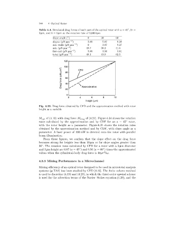
Fig. 4.33. Drag force obtained by CFD and the approximation method with rotor
height as a variable

M opt of (4.10) with dragforce M drag of (4.21). Figure 4.34 shows the rotation
rates calculated by the approximation and by CDF for an a =45 rotor,
◦
with the rotor height as a parameter. Figure 4.35 shows the rotation rates
obtained by the approximation method and by CDF, with slope angle as a
parameter. A laser power of 100 mW is directed onto the rotor with parallel
beam illumination.
From these figures, we confirm that the slope effect on the drag force
becomes strongfor heights less than 10 µm or for slope angles greater than
30 . The rotation rates calculated by CFD for a rotor with a 3 µm diameter
◦
and 3 µm height are 0.67 (a =45 ) and 0.56 (a =60 ) times the approximated
◦
◦
2
values when the cylindrical-body dragforce is 4πµr hω.
4.3.3 Mixing Performance in a Microchannel

Mixingefficiency of an optical rotor designed to be used in micrototal analysis
systems (µ-TAS) has been studied by CFD [4.13]. The finite volume method
is used to discretize (4.19) and (4.20), in which the third-order upwind scheme
is used for the advection terms of the Navier–Stokes equation (4.20), and the