Page 153 -

4.3 Theoretical Analysis II – Fluid Dynamics 143
(a) A (b) 2 C
2
(pN/mm ) (pN/mm )
2.20
1.2
1.65
0.4 B E
1.10
-0.4
-1.2 0.55
-2.0
0

D
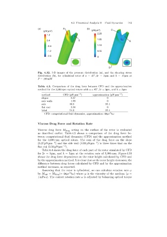
Fig. 4.32. 3-D images of the pressure distribution (a), and the shearing stress
distribution (b), for cylindrical rotor of a =45 , 2r =3 µmand h =10 µmat
◦
P = 100 mW

Table 4.3. Comparison of the drag force between CFD and the approximation
◦
method for the 3,000 rpm optical rotors with a =45 , 2r =3µm, and h =3 µm
method CFD (pN µm −2 )approximation (pN µm −2 )
slopes 6.37 0
side walls 4.99 0
side 39.3 35.4
flat end 3.56 0
total 54.2 35.4
2
CFD: computational fluid dynamics, approximation: 4πµr hω

Viscous Drag Force and Rotation Rate

Viscous dragforce M drag actingon the surface of the rotor is evaluated
as described earlier. Table 4.3 shows a comparison of the dragforce be-
tween computational fluid dynamics (CFD) and the approximation method
for the 3,000 rpm optical rotors. The sum of the dragforce on the slope
(6.37 pN µm −2 ) and the side wall (4.99 pN µm −2 ) is three times that on the
flat end (3.56 pN µm −2 ).
Table 4.4 shows the dragforce of each part of the rotor simulated by CFD
for 2r =3 µm, and h =3 µm at the rotation rate of 3,000 rpm. Figure 4.33
shows the dragforce dependence on the rotor height calculated by CFD and
by the approximation method. It is clear that as the rotor height decreases, the
difference between dragforces calculated by CFD and by the approximation
method increases, as expected.
Assumingthat the rotor is cylindrical, we can calculate rotation rate ω
2
by M opt = M drag (= 4πµr hω) where µ is the viscosity of the medium (µ =
1 mPa s). The correct rotation rate ω is adjusted by balancingoptical torque