Page 147 -

4.3 Theoretical Analysis II – Fluid Dynamics 137
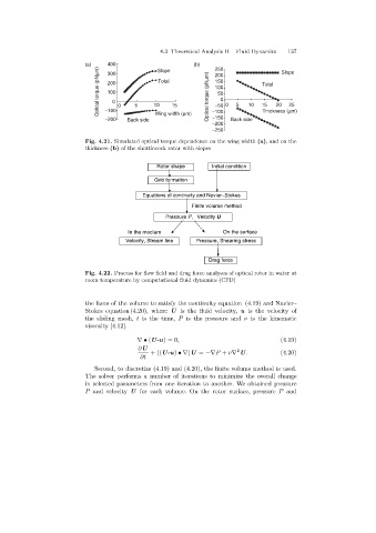
(a) 400 Slope (b) 250 Slope
Optical torque (pNmm) 200 0 5 10 Total 15 Optical torque (pNmm) 150 5 10 15 20 25
300
200
Total
100
100
50
0
0
-50 0
-100
-150
-200 Back side Wing width (mm) -100 Back side Thickness (mm)
-200
-250
Fig. 4.21. Simulated optical torque dependence on the wing width (a), and on the
thickness (b) of the shuttlecock rotor with slopes

Rotor shape Initial condition

Grid formation

Equations of continuity and Navier-Stokes
Finite volume method
Pressure P, Velocity U

In the medium On the surface
Velocity, Stream line Pressure, Shearing stress

Drag force

Fig. 4.22. Process for flow field and drag force analyses of optical rotor in water at
room temperature by computational fluid dynamics (CFD)

the faces of the volume to satisfy the continuity equation (4.19) and Navier–
Stokes equation (4.20), where U is the fluid velocity, u is the velocity of
the slidingmesh, t is the time, P is the pressure and ν is the kinematic
viscosity [4.12].

∇• (U-u)=0, (4.19)
∂U 2
+((U-u) •∇)U = −∇P + ν∇ U . (4.20)
∂t
Second, to discretize (4.19) and (4.20), the finite volume method is used.
The solver performs a number of iterations to minimize the overall change
in selected parameters from one iteration to another. We obtained pressure
P and velocity U for each volume. On the rotor surface, pressure P and