Page 165 - Modern Control Systems

Exercises 139

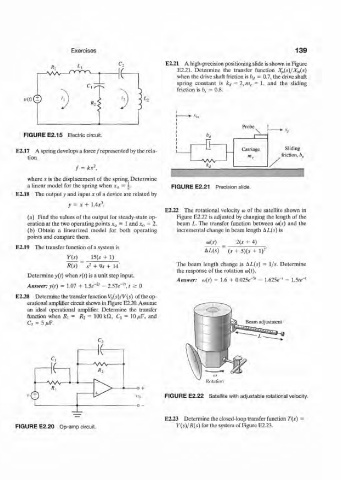
E2.21 A high-precision positioning slide is shown in Figure
E2.21. Determine the transfer function X p(s)/X m(s)
when the drive shaft friction is b d = 0.7, the drive shaft
spring constant is k d = 2, m c = 1, and the sliding
friction is b s = 0.8.
«(f)©

FIGURE E2.15 Electric circuit.

E2.17 A spring develops a force /represented by the rela- Sliding
tion friction, b.
2
/ = kx ,
where x is the displacement of the spring. Determine
a linear model for the spring when x 0 = - FIGURE E2.21 Precision slide.
j
E2.18 The output y and input x of a device are related by
3
y = x + 1.4x .
E2.22 The rotational velocity &> of the satellite shown in
(a) Find the values of the output for steady-state op- Figure E2.22 is adjusted by changing the length of the
= = 2. beam L. The transfer function between <x)(s) and the
eration at the two operating points x 0 1 and x 0
(b) Obtain a linearized model for both operating incremental change in beam length AL(s) is
points and compare them.
w(s) 2{s + 4)
E2.19 The transfer function of a system is 2
AZ-(.v) ( s + 5)(s + 1)
Y(s) _ 15(.f + 1)
R(s) ~ s 2 + 9s + 14' The beam length change is AL(i) = 1/s. Determine
the response of the rotation co(t).
Determine y{t) when r(t) is a unit step input.
5
Answer: «(r) = 1.6 + 0.025e~ ' - 1.625«-' - 1.5te ' -
-7
-
l
Answer: y(t) = 1.07 + i e * - 2.57e ', t s 0
E2.20 Determine the transfer function V Q(s)/V{s) of the op-
erational amplifier circuit shown in Figure E2.20. Assume
an ideal operational amplifier. Determine the transfer
function when /?, = R 2 = 100 kfl, C x = 10 jttF, and
= 5 fiF.
C 2
C,
-1(-

i^l'
Rotation
•t -o — FIGURE E2.22 Satellite with adjustable rotational velocity.
o +
*

E2.23 Determine the closed-loop transfer function T(s) =
FIGURE E2.20 Op-amp circuit. Y(s)/R(s) for the system of Figure E2.23.