Page 166 - Modern Control Systems

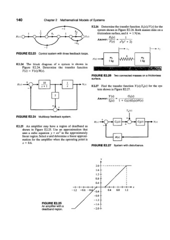
140 Chapter 2 Mathematical Models of Systems

E2.26 Determine the transfer function X 2(s)/F(s) for the
system shown in Figure E2.26. Both masses slide on a
frictionless surface, and k = 1 N/m.
/?(.v) O — • • X 2(s) 1
Answer: 2 2
F(s) s (s + 2)

FIGURE E2.23 Control system with three feedback loops.
/•*(/) MA/W-
E2.24 The block diagram of a system is shown in
Figure E2.24. Determine the transfer function
T(s) = Y(s)/R(s).
FIGURE E2.26 Two connected masses on a frictionless
surface.
10
R(s) • • Y(s)
s+ 1 E2.27 Find the transfer function Y(s)/T d(s) for the sys-
tem shown in Figure E2.27.
Y(s) G^s)
Answer:
T d(s) 1 + G,(s)G 2(s)H(s)

•O TAs)
FIGURE E2.24 Multiloop feedback system.
> * C,(s) - & * G 2{s) Yis)
E2.25 An amplifier may have a region of deadband as
shown in Figure E2.25. Use an approximation that
uses a cubic equation y = ax 3 in the approximately
linear region. Select a and determine a linear approxi-
H(s)
mation for the amplifier when the operating point is
JC = 0.6.
FIGURE E2.27 System with disturbance.

FIGURE E2.25
An amplifier with a
deadband region.