Page 173 - Organic Electronics in Sensors and Biotechnology

150 Cha pte r F o u r

Voltage response Current response
1 MΩ
10 MΩ
10 0
100 MΩ
1 GΩ
10 –1 10 –7 10 GΩ
100 GΩ
Voltage (V) 10 –2 Current (A)
1 MΩ
10 –3
10 MΩ
100 MΩ
10 –4 1 GΩ
10 GΩ
100 GΩ 10 –8
10 –5
10 –4 10 –2 10 0 10 2 10 4 10 6 10 –4 10 –2 10 0 10 2 10 4 10 6
Frequency (Hz) Frequency (Hz)
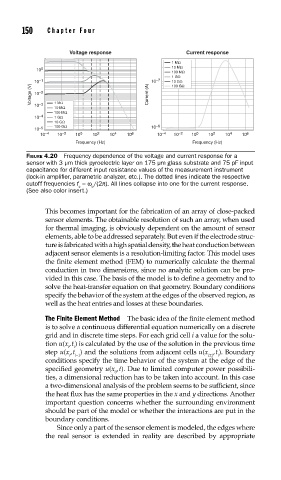
FIGURE 4.20 Frequency dependence of the voltage and current response for a
sensor with 3 μm thick pyroelectric layer on 175 μm glass substrate and 75 pF input
capacitance for different input resistance values of the measurement instrument
(lock-in amplifi er, parametric analyzer, etc.). The dotted lines indicate the respective
cutoff frequencies f =ω /(2π). All lines collapse into one for the current response.
c c
(See also color insert.)
This becomes important for the fabrication of an array of close-packed
sensor elements. The obtainable resolution of such an array, when used
for thermal imaging, is obviously dependent on the amount of sensor
elements, able to be addressed separately. But even if the electrode struc-
ture is fabricated with a high spatial density, the heat conduction between
adjacent sensor elements is a resolution-limiting factor. This model uses
the finite element method (FEM) to numerically calculate the thermal
conduction in two dimensions, since no analytic solution can be pro-
vided in this case. The basis of the model is to define a geometry and to
solve the heat-transfer equation on that geometry. Boundary conditions
specify the behavior of the system at the edges of the observed region, as
well as the heat entries and losses at these boundaries.

The Finite Element Method The basic idea of the finite element method
is to solve a continuous differential equation numerically on a discrete
grid and in discrete time steps. For each grid cell i a value for the solu-
tion u(x, t) is calculated by the use of the solution in the previous time
i i
step u(x, t ) and the solutions from adjacent cells u(x , t). Boundary
i i−1 i±1 i
conditions specify the time behavior of the system at the edge of the
specified geometry u(x , t). Due to limited computer power possibili-
0
ties, a dimensional reduction has to be taken into account. In this case
a two-dimensional analysis of the problem seems to be sufficient, since
the heat flux has the same properties in the x and y directions. Another
important question concerns whether the surrounding environment
should be part of the model or whether the interactions are put in the
boundary conditions.
Since only a part of the sensor element is modeled, the edges where
the real sensor is extended in reality are described by appropriate