Page 174 - Organic Electronics in Sensors and Biotechnology

Integrated Pyr oelectric Sensors 151

boundary conditions. The boundaries, where a heat transfer to the
environment takes place, were taken into account in the boundary con-
ditions as well, using the heat transfer coefficients from the one dimen-
sional model.
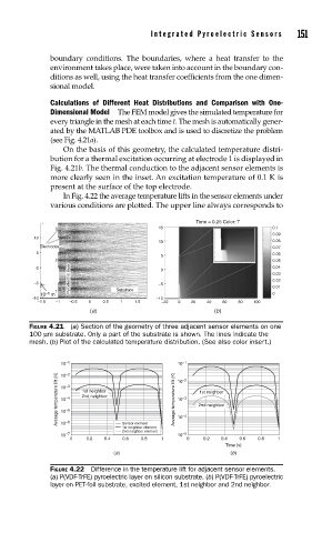
Calculations of Different Heat Distributions and Comparison with One-
Dimensional Model The FEM model gives the simulated temperature for
every triangle in the mesh at each time t. The mesh is automatically gener-
ated by the MATLAB PDE toolbox and is used to discretize the problem
(see Fig. 4.21a).
On the basis of this geometry, the calculated temperature distri-
bution for a thermal excitation occurring at electrode 1 is displayed in
Fig. 4.21b. The thermal conduction to the adjacent sensor elements is
more clearly seen in the inset. An excitation temperature of 0.1 K is
present at the surface of the top electrode.
In Fig. 4.22 the average temperature lifts in the sensor elements under
various conditions are plotted. The upper line always corresponds to

Time = 0.25 Color: T
3 15 0.1
2 0.09
10
10 0.08
Electrodes 0.07
5 0.06
5 1
2 0.05
Pyroelectric layer 0.02
0 0 0.04
0.03
–5 –5 0.01
1 Substrate
–6
10 m 0
–10 –10
–1.5 –1 –0.5 0 0.5 1 1.5 –20 0 20 40 60 80 100
(a) (b)
FIGURE 4.21 (a) Section of the geometry of three adjacent sensor elements on one
100 μm substrate. Only a part of the substrate is shown. The lines indicate the
mesh. (b) Plot of the calculated temperature distribution. (See also color insert.)
10 –1 10 –1
Average temperature lift (K) 10 –3 1st neighbor Average temperature lift (K) 10 –3 2nd neighbor
10 –2
10 –2
1st neighbor
2nd neighbor
10 –4
10 –5
10 –6
Sensor element
1st neighbor element 10 –4
2nd neighbor element
10 –7 10 –5
0 0.2 0.4 0.6 0.8 1 0 0.2 0.4 0.6 0.8 1
Time (s)
(a) (b)
FIGURE 4.22 Difference in the temperature lift for adjacent sensor elements.
(a) P(VDF-TrFE) pyroelectric layer on silicon substrate. (b) P(VDF-TrFE) pyroelectric
layer on PET-foil substrate, excited element, 1st neighbor and 2nd neighbor.