Page 208 - Renewable Energy Devices and System with Simulations in MATLAB and ANSYS

Power Electronics and Controls for Large Wind Turbines and Wind Farms 195

The value of C can be numerically approximated [71] by Equations 8.2 and 8.3. The values
p
C −C are related to the design of the WT rotor and can be decided depending on the aerodynamic
6
1
performance of selected WTs. These values can be found in Section 8.6.5.
 1  C 6 1
C p = C C 2 − C 3 θ p − C 4 θ C x C e i λ (8.2)
p −


5
1
 i λ 
1 1 0 035
.
= − 3 (8.3)
008 p θ
λ i λ + . θ p + 1
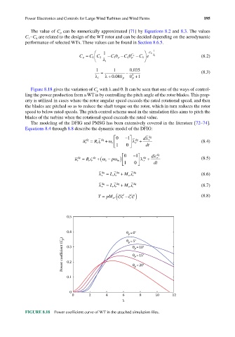
Figure 8.18 gives the variation of C with λ and θ. It can be seen that one of the ways of control-
p
ling the power production from a WT is by controlling the pitch angle of the rotor blades. This prop-
erty is utilized in cases where the rotor angular speed exceeds the rated rotational speed, and then
the blades are pitched so as to reduce the shaft torque on the rotor, which in turn reduces the rotor
speed to below rated speeds. The pitch control scheme used in the simulation files aims to pitch the
blades of the turbine when the rotational speed exceeds the rated value.
The modeling of the DFIG and PMSG has been extensively covered in the literature [72–74].
Equations 8.4 through 8.8 describe the dynamic model of the DFIG:
0 −  1 dλ dq
s +
u s = R ss i dq + ω s   λ dq s (8.4)
dq
 1 0  dt
0 −  1 dλ dq
dq
dq
dq
u r = R rr +(ω s − ω m  λ r + r (8.5)
i
p ) 
 1 0  dt
dq
λ s = L s s i dq + M sr r i dq (8.6)
dq
λ r = L r r i dq + M sr s i dq (8.7)
d q
q d
T = pM sr( ii r − ) (8.8)
s
s ii r
0.5

0.4 θ =0°
p
Power coefficient (C p ) 0.3 θ =10°
θ =5°
p
p
=15°
θ p
0.2
θ =20°
0.1 p

0
0 2 4 6 8 10 12
λ

FIGURE 8.18 Power coefficient curve of WT in the attached simulation files.