Page 258 - Renewable Energy Devices and System with Simulations in MATLAB and ANSYS

Electric Generators and their Control for Large Wind Turbines 245

jq
ω r P <0
S
i q <0
–R i
S S
V SO
δ v
ω r
i
i d L dm F d
δ v L i
d d
ji q ψ jL i
q q
i SO SO
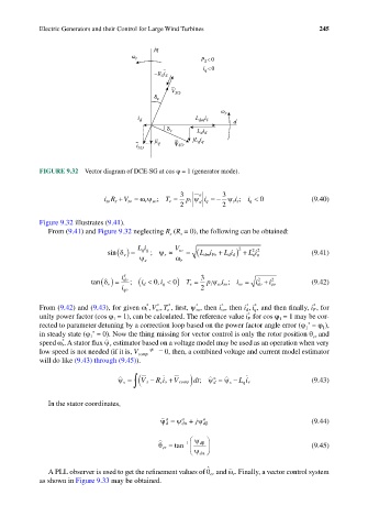
FIGURE 9.32 Vector diagram of DCE-SG at cos φ = 1 (generator mode).

3 a 3
iR s + V so = ωψ ; T e = p ψ i q = − ψ ; i q < 0 (9.40)
so
so
r
1
i s s
2 d 2
Figure 9.32 illustrates (9.41).
From (9.41) and Figure 9.32 neglecting R (R = 0), the following can be obtained:
s
s
Li V 2
sin δ v ( ) = qq ; ψ s ≈ so = ( Li Li Li (9.41)
dd) +
dm Fo +
22
qq
ψ s ω r
tan δ v ( ) = do i s ; ( d i < 0 , q i < ) 0 e T = 3 p 1 ψ soso i ; i = do i + 2 qo i (9.42)
2
so
qo i 2
*
*
*
*
*
*
*
*
d ,
,
From (9.42) and (9.43), for given ω 1 , VT e , first, ψ so , then i so , then ii q , and then finally, i F , for
so
*
unity power factor (cos φ = 1), can be calculated. The reference value i F for cos φ = 1 may be cor-
1
1
rected to parameter detuning by a correction loop based on the power factor angle error (φ − φ ),
*
1
1
*
in steady state (φ = 0). Now the thing missing for vector control is only the rotor position θ and
er
1

*
speed ω r . A stator flux ψ s estimator based on a voltage model may be used as an operation when very
low speed is not needed (if it is, V comp ≠− 0, then, a combined voltage and current model estimator
will do like (9.43) through (9.45)).
ψ s = ( s V − R s s i + V comp dt ) ; ψ d = ψ s − Li (9.43)

∫
a
q s
In the stator coordinates,
a
a
a
ψ d = ψ αd + j ψ βd (9.44)
 ψ β 
θ er = tan −1  d  (9.45)
 ψ αd 

ˆ
A PLL observer is used to get the refinement values of θ er and ω r . Finally, a vector control system
as shown in Figure 9.33 may be obtained.