Page 257 - Renewable Energy Devices and System with Simulations in MATLAB and ANSYS

244 Renewable Energy Devices and Systems with Simulations in MATLAB and ANSYS ®
®

1.2 l e =l e0 , l s =0
, l =ln
l =l e0max s
e
0.8
0.4
Flux density (T) –0.4 0

–0.8

–1.2
0 1 2 3 4 5 6
(c) Electrical angle (rad)

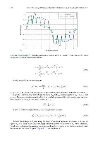
FIGURE 9.31 (Continued ) FEM key validation on optimal design of 7.6 MW, 11 rpm DCE-SG: (c) radial
air-gap flux density (at no load and full load).

2  j 2π − j 2π 
V s =  V a + e 3 V b + e 3 V c ⋅ e − θ
j er
3     (9.36)
2  j 2π − j 2 2π 
I s =   I a + e 3 I b + e 3 I c ⋅ e − θ j er

3  
Finally, the field circuit equations are

dψ s
s
s
iR F − V F = − F ; ψ s F = Li F + L dm( i d + ) (9.37)
s
s
lF
F
i F
dt
s
s
s
s
s
V RL lF ,, ψ are all reduced to the stator by a transformation (equivalent turns ratio) coefficient k .
F ,
F ,
F
i F
F
s
Magnetic saturation may be modeled mainly by L and L , which depend on i = i + i and
dm
qm
dm
d
F
i = i . The cross-coupling saturation has to be carefully considered for both steady-state and tran-
q
qm
a
sient operation modes [4]. The active flux ψ is [23]
d
a
q s
ψ = ψ − Li (9.38)
s
d
It turns to be the multiplier to of i in the torque expression [23]
q
dm F −(
a
a
ψ =  Li d L − )  ; e T = 3 p 1 ψ i q (9.39)
q L
d i
d   2 d
But this flux linkage is aligned along the d-axis of the rotor, and thus, its position is θ and its
er
= ˆ ω r at all loads. Cross-coupling saturation introduces an error to θ , when estimated,
speed ˆ ω ψ d er
which may be handled by adding a correction angle Δθ . For unity power factor, the steady-state
er
equations and the vector diagram (Figure 9.32) are simplified to