Page 191 - Schaum's Outline of Theory and Problems of Electric Circuits

HIGHER-ORDER CIRCUITS AND COMPLEX FREQUENCY
180
[CHAP. 8
4
2ðs þ 1Þ 2
s s þ 3s þ 4
Z in ðsÞ¼ 2 þ ¼ð2Þ
4 s þ s þ 2
2
2ðs þ 1Þþ
s
(a) Z in ð0Þ¼ 4
, the impedance offered to a constant (dc) source in the steady state.
2
ð j4Þ þ 3ð j4Þþ 4
ðbÞ Z in ð j4Þ¼ 2 ¼ 2:33 29:058
2
ð j4Þ þ j4 þ 2
This is the impedance offered to a source sin 4t or cos 4t.
(c) Z in ð1Þ ¼ 2
. At very high frequencies the capacitance acts like a short circuit across the RL branch.

8.12 Express the impedance ZðsÞ of the parallel combination of L ¼ 4 H and C ¼ 1 F. At what
frequencies s is this impedance zero or infinite?

ð4sÞð1=sÞ s
ZðsÞ¼ ¼
2
4s þð1=sÞ s þ 0:25
By inspection, Zð0Þ¼ 0 and Zð1Þ ¼ 0, which agrees with our earlier understanding of parallel LC circuits at
frequencies of zero (dc) and infinity. For jZðsÞj ¼ 1,
2
s þ 0:25 ¼ 0 or s ¼ j0:5 rad=s
A sinusoidal driving source, of frequency 0.5 rad/s, results in parallel resonance and an infinite impedance.

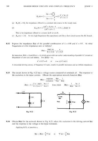
8.13 The circuit shown in Fig. 8-22 has a voltage source connected at terminals ab. The response to
the excitation is the input current. Obtain the appropriate network function HðsÞ.
response IðsÞ 1
HðsÞ¼ ¼
excitation VðsÞ ZðsÞ
ð2 þ 1=sÞð1Þ 8s þ 3 1 3s þ 1
ZðsÞ¼ 2 þ ¼ from which HðsÞ¼ ¼
2 þ 1=s þ 1 3s þ 1 ZðsÞ 8s þ 3

Fig. 8-22 Fig. 8-23

8.14 Obtain HðsÞ for the network shown in Fig. 8-23, where the excitation is the driving current IðsÞ
and the response is the voltage at the input terminals.
Applying KCL at junction a,

s 0 0 15
IðsÞþ 2IðsÞ¼ V ðsÞ or V ðsÞ¼ IðsÞ
5 s