Page 192 - Schaum's Outline of Theory and Problems of Electric Circuits

HIGHER-ORDER CIRCUITS AND COMPLEX FREQUENCY
CHAP. 8]
At the input terminals, KVL gives 181

0 15
VðsÞ¼ 2sIðsÞþ V ðsÞ¼ 2s þ IðsÞ
s
2
VðsÞ 2s þ 15
Then HðsÞ¼ ¼
IðsÞ s

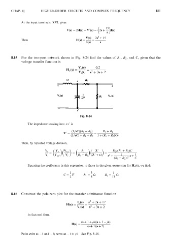
8.15 For the two-port network shown in Fig. 8-24 find the values of R 1 , R 2 , and C, given that the
voltage transfer function is
V o ðsÞ 0:2
H v ðsÞ ¼ 2
V i ðsÞ s þ 3s þ 2

Fig. 8-24
0
The impedance looking into xx is
ð1=sCÞðR 1 þ R 2 Þ
0 R 1 þ R 2
Z ¼ ¼
ð1=sCÞþ R 1 þ R 2 1 þðR 1 þ R 2 ÞCs
Then, by repeated voltage division,
0
V o V o V xx 0 R 2 Z R 2 =ðR 1 þ R 2 ÞC
¼ ¼ 0 ¼
2
V i V xx 0 V i R 1 þ R 2 Z þ s1 s þ 1 s þ 1
ðR 1 þ R 2 ÞC C
Equating the coefficients in this expression to those in the given expression for H v ðsÞ, we find:

1 3 1
C ¼ F R 1 ¼
R 2 ¼
2 5 15

8.16 Construct the pole-zero plot for the transfer admittance function

2
I o ðsÞ s þ 2s þ 17
HðsÞ¼ ¼ 2
V i ðsÞ s þ 3s þ 2
In factored form,

ðs þ 1 þ j4Þðs þ 1 j4Þ
HðsÞ¼
ðs þ 1Þðs þ 2Þ
Poles exist at 1 and 2; zeros at 1 j4. See Fig. 8-25.