Page 50 - Statistics for Environmental Engineers

L1592_Frame_C04 Page 42 Tuesday, December 18, 2001 1:41 PM

For example, the BOD discharged into a freely flowing stream is important the day it is discharged. A
2- or 3-day average might also be important because a few days of dissolved oxygen depression could
be disastrous while one day might be tolerable to aquatic organisms. A 30-day average of BOD could
be a less informative statistic about the threat to fish than a short-term average, but it may be needed to
assess the long-term trend in treatment plant performance.
For suspended solids that settle on a stream bed and form sludge banks, a long-term average might
be related to depth of the sludge bed and therefore be an informative statistic. If the solids do not settle,
the daily values may be more descriptive of potential damage. For a pollutant that could be ingested by
an organism and later excreted or metabolized, the exponentially weighted moving average might be a
good statistic.
Conversely, some pollutants may not exhibit their effect for years. Carcinogens are an example where
the long-term average could be important. Long-term in this context is years, so the 30-day average would
not be a particularly useful statistic. The first ingested (or inhaled) irritants may have more importance
than recently ingested material. If so, perhaps past events should be weighted more heavily than recent
events if a statistic is to relate source of pollution to present effect. Choosing a statistic with the
appropriate weighting could increase the value of the data to biologists, epidemiologists, and others who
seek to relate pollutant discharges to effects on organisms.

Plotting on a Logarithmic Scale
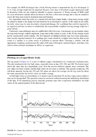
The top panel of Figure 4.1 is a plot of influent copper concentration at a wastewater treatment plant.
This plot emphasizes the few high values, expecially those at days 225, 250, and 340. The bottom panel
shows the same data on a logarithmic scale. Now the process behavior appears more consistent. The
low values are more evident, and the high values do not seem so extreme. The episode around day 250
still looks unusual, but the day 225 and 340 values are above the average (on the log scale) by about
the same amount that the lowest values are below average.
Are the high values so extraordinary as to deserve special attention? Or are they rogue values (outliers)
that can be disregarded? This question cannot be answered without knowing the underlying distribution
of the data. If the underlying process naturally generates data with a lognormal distribution, the high
values fit the general pattern of the data record.

1000
Copper (mg/L) 500

0
10000
Copper (mg/L) 1000

100
10
0 50 100 150 200 250 300 350
Days

FIGURE 4.1 Copper data plotted on arithmetic and logarithmic scales give a different impression about the high values.
© 2002 By CRC Press LLC