Page 54 - Statistics for Environmental Engineers

L1592_Frame_C04 Page 46 Tuesday, December 18, 2001 1:41 PM

Missing values in the data series might seem to be a barrier to smoothing, but for practical purposes
they usually can be filled in using some simple ad hoc method. For purposes of smoothing to clarify
the general trend, several methods of filling in missing values can be used. The simplest is linear
interpolation between adjacent points. Other alternatives are to fill in the most recent moving average
value, or to replicate the most recent observation. The general trend will be nearly the same regardless
of the choice of method, and the user should not be unduly worried about this so long as missing values
occur only occasionally.

References
Box, G. E. P., G. M. Jenkins, and G. C. Reinsel (1994). Time Series Analysis, Forecasting and Control, 3rd
ed., Englewood Cliffs, NJ, Prentice-Hall.
Chatfield, C. (1988). Problem Solving: A Statistician’s Guide, London, Chapman & Hall.
Chatfield, C. (1991). “Avoiding Statistical Pitfalls,” Stat. Sci., 6(3), 240–268.
Cryer, J. D. (1986). Time Series Analysis, Duxbury Press, Boston.
Tukey, J. W. (1977). Exploratory Data Analysis, Reading, MA, Addison-Wesley.

Exercises

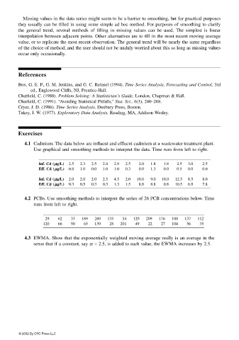
4.1 Cadmium. The data below are influent and effluent cadmium at a wastewater treatment plant.
Use graphical and smoothing methods to interpret the data. Time runs from left to right.

Inf. Cd (µµ µµg/L) 2.5 2.3 2.5 2.8 2.8 2.5 2.0 1.8 1.8 2.5 3.0 2.5
Eff. Cd (µµ µµg/L) 0.8 1.0 0.0 1.0 1.0 0.3 0.0 1.3 0.0 0.5 0.0 0.0
Inf. Cd (µµ µµg/L) 2.0 2.0 2.0 2.5 4.5 2.0 10.0 9.0 10.0 12.5 8.5 8.0
Eff. Cd (µµ µµg/L) 0.3 0.5 0.3 0.3 1.3 1.5 8.8 8.8 0.8 10.5 6.8 7.8

4.2 PCBs. Use smoothing methods to interpret the series of 26 PCB concentrations below. Time
runs from left to right.

29 62 33 189 289 135 54 120 209 176 100 137 112
120 66 90 65 139 28 201 49 22 27 104 56 35

4.3 EWMA. Show that the exponentially weighted moving average really is an average in the
sense that if a constant, say α = 2.5, is added to each value, the EWMA increases by 2.5.

© 2002 By CRC Press LLC