Page 56 - Statistics for Environmental Engineers

L1592_Frame_C05 Page 48 Tuesday, December 18, 2001 1:42 PM

TABLE 5.1
BOD Data from an Industrial Survey
Date 4 am 8 am 12 N 4 pm 8 pm 12 MN
2/10 717 946 623 490 666 828
2/11 1135 241 396 1070 440 534
2/12 1035 265 419 413 961 308
2/13 1174 1105 659 801 720 454
2/14 316 758 769 574 1135 1142
2/15 505 221 957 654 510 1067
2/16 329 371 1081 621 235 993
2/17 1019 1023 1167 1056 560 708
2/18 340 949 940 233 1158 407
2/19 853 754 207 852 318 358
2/20 356 847 711 1185 825 618
2/21 454 1080 440 872 294 763
2/22 776 502 1146 1054 888 266
2/23 619 691 416 1111 973 807
2/24 722 368 686 915 361 346
2/25 1110 374 494 268 1078 481
2/26 472 671 556 — — —
Source: U.S. EPA (1973). Monitoring Industrial Wastewater,
Washington, D.C.

1500
BOD Concentration (mg/L) 1000
1250

750

500
250
0
0 20 40 60 80 100
Observation (at 4-hour intervals)

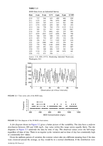
FIGURE 5.1 Time series plot of the BOD data.

5 4
Frequency 3 2

0 1
200 400 600 800 1000 1200
BOD Concentration (mg/L)

FIGURE 5.2 Dot diagram of the 99 BOD observations.

A dot diagram shown in Figure 5.2 gives a better picture of the variability. The data have a uniform
distribution between 200 and 1200 mg/L. Any value within this range seems equally likely. The dot
diagrams in Figure 5.3 subdivide the data by time of day. The observed values cover the full range
regardless of time of day. There is no regular cyclic variation and no time of day has consistently high
or consistently low values.
Given the uniform pattern of variation, the extreme values take on a different meaning than if the data
were clustered around the average, as they would be in a normal distribution. If the distribution were
© 2002 By CRC Press LLC