Page 57 - Statistics for Environmental Engineers

L1592_Frame_C05 Page 49 Tuesday, December 18, 2001 1:42 PM

4 am
8 am
Time of Day 4 pm
12 N

8 pm

12 MN
200 400 600 800 1000 1200
BOD Concentration, mg/L

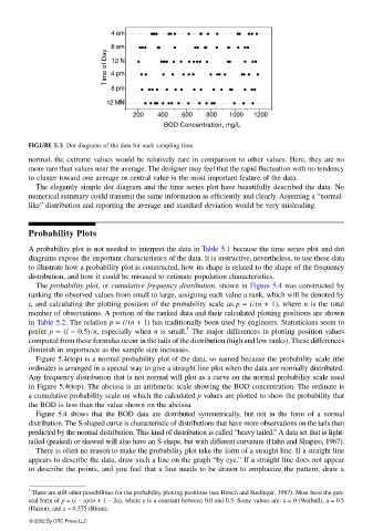
FIGURE 5.3 Dot diagrams of the data for each sampling time.

normal, the extreme values would be relatively rare in comparison to other values. Here, they are no
more rare than values near the average. The designer may feel that the rapid fluctuation with no tendency
to cluster toward one average or central value is the most important feature of the data.
The elegantly simple dot diagram and the time series plot have beautifully described the data. No
numerical summary could transmit the same information as efficiently and clearly. Assuming a “normal-
like” distribution and reporting the average and standard deviation would be very misleading.

Probability Plots

A probability plot is not needed to interpret the data in Table 5.1 because the time series plot and dot
diagrams expose the important characteristics of the data. It is instructive, nevertheless, to use these data
to illustrate how a probability plot is constructed, how its shape is related to the shape of the frequency
distribution, and how it could be misused to estimate population characteristics.
The probability plot, or cumulative frequency distribution, shown in Figure 5.4 was constructed by
ranking the observed values from small to large, assigning each value a rank, which will be denoted by
i, and calculating the plotting position of the probability scale as p = i/(n + 1), where n is the total
number of observations. A portion of the ranked data and their calculated plotting positions are shown
in Table 5.2. The relation p = i/(n + 1) has traditionally been used by engineers. Statisticians seem to
1
prefer p = (i − 0.5)/n, especially when n is small. The major differences in plotting position values
computed from these formulas occur in the tails of the distribution (high and low ranks). These differences
diminish in importance as the sample size increases.
Figure 5.4(top) is a normal probability plot of the data, so named because the probability scale (the
ordinate) is arranged in a special way to give a straight line plot when the data are normally distributed.
Any frequency distribution that is not normal will plot as a curve on the normal probability scale used
in Figure 5.4(top). The abcissa is an arithmetic scale showing the BOD concentration. The ordinate is
a cumulative probability scale on which the calculated p values are plotted to show the probability that
the BOD is less than the value shown on the abcissa.
Figure 5.4 shows that the BOD data are distributed symmetrically, but not in the form of a normal
distribution. The S-shaped curve is characteristic of distributions that have more observations on the tails than
predicted by the normal distribution. This kind of distribution is called “heavy tailed.” A data set that is light-
tailed (peaked) or skewed will also have an S-shape, but with different curvature (Hahn and Shapiro, 1967).
There is often no reason to make the probability plot take the form of a straight line. If a straight line
appears to describe the data, draw such a line on the graph “by eye.” If a straight line does not appear
to describe the points, and you feel that a line needs to be drawn to emphasize the pattern, draw a

1
There are still other possibilities for the probability plotting positions (see Hirsch and Stedinger, 1987). Most have the gen-
eral form of p = (i − a)/(n + 1 − 2a), where a is a constant between 0.0 and 0.5. Some values are: a = 0 (Weibull), a = 0.5
(Hazen), and a = 0.375 (Blom).
© 2002 By CRC Press LLC