Page 248 - Sustainability in the Process Industry Integration and Optimization

E x a m p l e s a n d Ca s e S t u d i e s 225

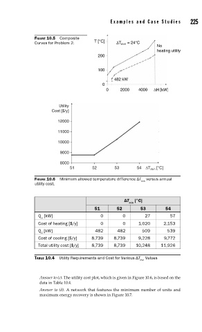
FIGURE 10.5 Composite
Curves for Problem 2. T [°C] ΔT min = 24°C
No
heating utility
200

100

482 kW
0
0 2000 4000 ΔH [kW]

Utility
Cost [$/y]

12000
11000

10000

9000
8000
51 52 53 54 ΔT min [°C]

FIGURE 10.6 Minimum allowed temperature difference ΔT versus annual
min
utility cost.

ΔT [°C]
min
51 52 53 54
Q [kW] 0 0 27 57
H
Cost of heating [$/y] 0 0 1,020 2,153
Q [kW] 482 482 509 539
C
Cost of cooling [$/y] 8,739 8,739 9,228 9,772
Total utility cost [$/y] 8,739 8,739 10,248 11,926

TABLE 10.4 Utility Requirements and Cost for Various ΔT Values
min

Answer to (c). The utility cost plot, which is given in Figure 10.6, is based on the
data in Table 10.4.
Answer to (d). A network that features the minimum number of units and
maximum energy recovery is shown in Figure 10.7.