Page 265 - The Combined Finite-Discrete Element Method

248 TRANSITION FROM CONTINUA TO DISCONTINUA

(a) (b) (c)

(d) (e) (f)

(g) (h) (i)

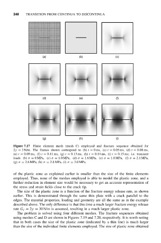
Figure 7.17 Finite element mesh (mesh C) employed and fracture sequence obtained for
2γ = 3 N/m. The frames shown correspond to (b) t = 0ms, (c) t = 0.05 ms, (d) t = 0.08 ms,
(e) t = 0.09 ms, (f) t = 0.11 ms, (g) t = 0.13 ms, (h) t = 0.14 ms, (i) t = 0.15 ms; i.e. transient
loads (b) σ = 0MPa, (c) σ = 1.0MPa, (d) σ = 1.6MPa, (e) σ = 1.8 MPa, (f) σ = 2.1MPa,
(g) σ = 2.6MPa, (h) σ = 2.8MPa, (i) σ = 3.0MPa.

of the plastic zone as explained earlier is smaller than the size of the finite elements
employed. Thus, none of the meshes employed is able to model the plastic zone, and a
further reduction in element size would be necessary to get an accurate representation of
the stress and strain fields close to the crack tip.
The size of the plastic zone is a function of the fracture energy release rate, as shown
earlier. This is demonstrated through the same thin plate with a crack parallel to the
edges. The material properties, loading and geometry are all the same as in the example
described above. The only difference is that this time a much larger fracture energy release
rate G f = 2γ = 30 N/m is assumed, resulting in a much larger plastic zone.
The problem is solved using four different meshes. The fracture sequences obtained
using meshes C and D are shown in Figures 7.19 and 7.20, respectively. It is worth noting
that in both cases the size of the plastic zone (indicated by a thin line) is much larger
than the size of the individual finite elements employed. The size of plastic zone obtained