Page 266 - The Combined Finite-Discrete Element Method

DISCRETE CRACK MODEL 249

(a) (b) (c)

(d) (e) (f)

(g) (h) (i)

(j) (k) (l)

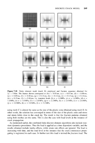
Figure 7.18 Finite element mesh (mesh D) employed and fracture sequence obtained for
2γ = 3 N/m. The frames shown correspond to (b) t = 0.05 ms, (c) t = 0.07 ms, (d) t = 0.08 ms,
(e) t = 0.09 ms, (f) t = 0.10 ms, (g) t = 0.11 ms, (h) t = 0.12 ms, (i) t = 0.13 ms, (j) t = 0.14 ms,
(k) t = 0.15 ms, (l) t = 0.16 ms; i.e. transient loads (b) σ = 1.0MPa, (c) σ = 1.4MPa, (d) σ =
1.6MPa, (e) σ = 1.8 MPa, (f) σ = 2.0MPa, (g) σ = 2.2MPa, (h) σ = 2.4MPa, (i) σ = 2.6MPa,
(j) σ = 2.8MPa, (k) σ = 3.0MPa, (l) σ = 3.2MPa.

using mesh C is almost the same as the size of the plastic zone obtained using mesh D. In
other words, the solution has converged in terms of the size of the plastic zone and stress
and strain fields close to the crack tip. The result is that the fracture patterns obtained
using both meshes are the same. This is also the case with load levels at the instance of
crack propagation.
As mentioned earlier, the combined finite-discrete element algorithms also include tran-
sient dynamics procedures. Thus the load is applied as a time dependent variable, and the
results obtained include inertia effects, while strain rate effects are ignored. The load is
increasing with time, and the load level at the instance that the crack commences propa-
gating is registered in each case. In further text this load is termed the fracture load.The