Page 112 - The Geological Interpretation of Well Logs

- THE GEOLOGICAL INTERPRETATION OF WELL LOGS -

specific stratigraphic intervals, especially in fine grained INTERVAL
TRANSIT TIME
sequences. There are many examples in the literature (i.e.
(microseconds) o
Michelsen, 1989; Whittaker e7 af, 1985).
240 40| 3
L L 1 1 oO

Fracture identification =
F
A knowledge of the presumed travel paths of the sonic -l
signals (Figure 8.7) suggests that the log may be used for 4004
fracture identification. The sonic log porosity is probably
only that due to the matrix, and does not include fracture
porosity. This is because the sonic pulse will follow the
fastest path to the receiver and this will avoid fractures.
5007
Comparing sonic porosity to global porosity should
indicate zones of fracture. The subject is fully described
under the Density Log (see Chapter 9, ‘Fracture identifi-
cation’). The use of the full waveform acoustic log in
-~ 600;
fracture analysis is discussed below (Section 8.8). € tc
~ < <
s & f 5
Compaction
3 ° wi
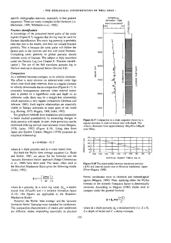
As a sediment becomes compact, so its velocity increases. . < re
The effect is most obvious on reduced-scale sonic logs 7004 Sf ws
& =
where, over thick shale intervals, there is a regular increase °
al
in velocity downwards due to compaction (Figure 8.17). In
extremely homogeneous intervals when interval transit
time is plotted on a Jogarithmic scale and depth on an 800
-
arithmetic scale, there may be a straight-line relationship
which represents a very regular compaction (Hottman and
Johnson, 1965). Such regular relationships are especially
visible in Tertiary sediments in many parts of the world 9007
(e.g. Herring, 1973; Magara, 1968; Issler, 1992).
But graphical methods have limitations and compaction
is better studied quantitatively by measuring changes in
Figure 8.17 Compaction in a shale sequence shown by a
shale porosity with depth. In turn, shale porosities can be
regular decrease in interval transit me with depth. The
calibrated with log derived interval transit times (Magara,
velocity decreases from approximately 160p/ft to 140p/ft
1978; Issler, 1992) (Figure 8.18). Using data from over 500m.
Japan and Eastern Canada, Magara (1978) proposed an
empirica] relationship:
$%
6 = 0.466A0 - 31.7
POROSITY
where $ = shale porosity and Az = sonic transit time. —
But both the Wyllie time average equation (i.e, Bulat 2
160 160 140 130 120 1190 100 so 80 70
and Stoker, 1987, see above for the formula) and the
INTERVAL TRANSIT TIME At log pft
‘acoustic formation factor’ approach (Raiga-Clemenceau
et al., 1988) have been used. The latter, when used in Figure 8.18 The relationship between mudstone porosity
the Beaufort-Mackenzie Basin gives the following results ( &%) and interval transit time in Miocene mudstones, Japan.
(Issler, 1992): (From Magara, 1968).
Atma \1 forces, sandstones more to chemical and mineralogical
=1- _
¢ ( At iF agents (Magara, 1980). Thus, applying either the Wyilie
formula or the acoustic formation factor is theoretically
where ¢ = porosity, Ar = sonic log value, Ar, = matrix incorrect. According to Magara (1980) shales tend to
transit time (67ps/ft) and « = acoustic formation factor compact under the general formula:
(2.19), (the figures are applicable to the Beaufort-
Mackenzie Basin). (-Z)
=
exp
9 = bo exp ——
However, the Wyllie ‘time average’ and the “acoustic
formation factor’ formulae were intended for sandstones.
The compaction characteristics of shales and sandstones where ¢ = shale porosity, , = initial porosity (i.e. Z = 0),
are different, shales responding essentially to physical Z = depth of burial and C = decay constant.
102