Page 117 - The Geological Interpretation of Well Logs

- SONIC OR ACOUSTIC LOGS -

8.7 Seismic applications Interval velocities
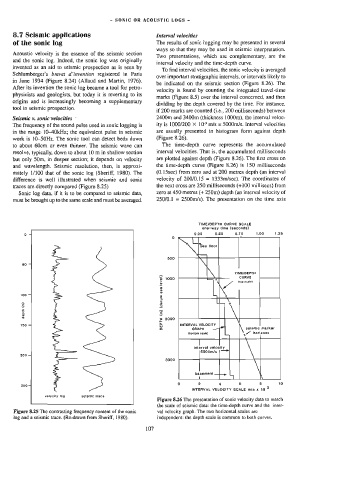
of the sonic log The results of sonic logging may be presented in several
ways so that they may be used in seismic interpretation.
Acoustic velocity is the essence of the seismic section
Two presentations, which are complementary, are the
and the sonic log. Indeed, the sonic log was originally
interval velocity and the time-depth curve.
invented as an aid to seismic prospection as is seen by
To find interval velocities, the sonic velocity is averaged
Schlumberger’s brevet d’invention registered in Paris
over important stratigraphic intervals, or intervals likely to
in June 1934 (Figure 8.24) (Allaud and Martin, 1976).
be indicated on the seismic section (Figure 8.26). The
After its invention the sonic log became a tool for petro-
velocity is found by counting the integrated travel-time
physicists and geologists, but today it is reverting to its
marks (Figure 8.5) over the interval concerned, and then
origins and is increasingly becoming a supplementary
dividing by the depth covered by the time. For instance.
tool in seismic prospection.
if 200 marks are counted (i.¢., 200 milliseconds) between
Seismic v. sonic velocities - 2400m and 3400m (thickness 1000m), the interval veloc-
The frequency of the sound pulse used in sonic logging is ity is 1000/200 X 10% m/s = 5000m/s. Interval] velocities
in the range. 1|O-40kHz; the equivalent pulse in seismic are usually presented in histogram form against depth
work is 10-50Hz. The sonic tool can detect beds down (Figure 8.26).
to about 60cm or even thinner. The seismic wave can The time-depth curve represents the accumulated
resolve, typically, down to about 10 m in shallow section interval velocities. That is, the accumulated milliseconds
but only 50m, in deeper section; it depends on velocity are plotted against depth (Figure 8.26). The first cross on
and wavelength. Seismic resolution, then, is approxi- the time-depth curve (Figure 8.26) is 150 milliseconds
mately 1/100 that of the sonic log (Sheriff, 1980). The (0.15sec) from zero and at 200 metres depth (an interval
difference is well illustrated when seismic and sonic velocity of 200/0.15 = 1333m/sec). The coordinates of
traces are directly compared (Figure 8.25) the next cross are 250 milliseconds (+100 millisecs) from
Sonic log data, if it is to be compared to seismic data, zero at 450 metres (+ 250m) depth (an interval velocity of
must be brought up to the same scale and must be averaged. 250/0.1 = 2500m/s). The presentation on the time axis

TIME/QGEPTH CURVE SCALE
one-way time (seconds)

0.25 0.50 0.75 1.00 1.25
0
Lh
\ a¢a floor

600
\

\ TIME/DEPTH

3. 1000 CURVE
=
3 x A (lop scale)
x
oo
»
3 1
x
I
5
(m)> 3 *
depth = \
z= 2000
V
~ a °o l & INTERVAL VELOCITY
S GRAPH _ \ seismic marker
(o0ttom scale) ae horizons
+

Interval velocily
|°oron"s ’
200

3000 \

L
basement —+_,
L
\
1
8
6
2
4
260 0 INTERVAL VELOCITY SCALE m/s x 10 3 10
velocity log
seismic race
the scale of seismic data: the time-depth curve and the inter-
Figure 8.26 The presentation of sonic velocity data to match
Figure 8,25 The contrasting frequency content of the sonic val velocity graph. The two horizontal scales are
log and a seismic trace. (Re-drawn from Sheriff, 1980). independent: the depth scale is common to both curves.
107