Page 114 - The Geological Interpretation of Well Logs

- THE GEOLOGICAL INTERPRETATION OF WELL LOGS -

sum of the hydrostatic pressure to D, and the lithostatic
At u/ft
pressure from D, to D.
180 149 100 80
Although the sonic log can be used to identify over-
1
L
4
L
1
1
lL
pressure, it can only do so once drilling and logging are 2790
completed, by which time it may be too late!
Borehole damage
The frequent comparison between seismic and sonic
velocities has shown that there are often differences
between the two which cannot be accounted for by
frequency difference (Figure 8.25). The differences are
thought to exist, at least partly, because sonic velocities
i
can be affected by mechanical or chemical damage 2800
immediately around the borehole. The very shallow depth
wn
of penetration of the sonic pulse has been discussed 2
Ss
(Section 8.4) which means that it is susceptible to imme- <=
wa
diate borehole conditions. Drilling can cause damage at
>
the borehole wall, especially to shales either mechanical- c
ly, by fracturing and spalling (Section 4.4}, or chemically oO
Ee P
by the (chemical) reaction of the drilling mud with the
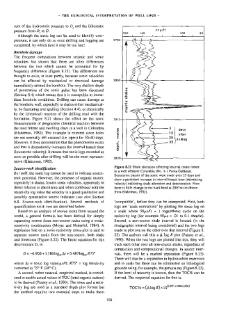
formation. Figure 8.21 shows the effect on the sonic
2810 +
measurements of progressive chemical reaction between
the mud filtrate and swelling clays in a well in Colombia wo
z
(Blakeman, 1982). The example is extreme since holes 2 after
are not normally left uncased (i.e. open) for 30-40 days. * 5 \ arilting
However, it does demonstrate that the phenomenon exists 2820
x=
-
and that it dramatically increases the interval transit time o® Qa
(lowers the velocity). It means that sonic logs recorded as oa
soon as possible after drilling will be the most represen-
tative (Blakeman, 1982).
Figure 8.21 Shale alteration affecting interval transit times
Source-rock identification
in a well offshore Columbia (No. 1-1 Punta Gallinas).
By itself, the sonic log cannot be used to indicate source-
Successive passes of the sonic were made over 35 days and
rock potential. However, the presence of organic matter,
show a persistent increase in interval transit time (decreasing
especially in shales, lowers sonic velocities, apparently in velocity) indicating shale alteration and deterioration. Note
direct relation to abundance and when combined with the there is little change in the hard band at 2807m (re-drawn
resistivity log value the velocity is a good qualitative and from Blakeman, 1982).
possibly quantitative source indicator (see also Section
6.8, Source-rock identification). Several methods of ‘compatible’, before they can be interpreted. First, both
quantification exist: two are described below. logs are ‘scale normalized’ by plotting the sonic log on
Based on an analysis of source rocks from around the a scale where S5Ous/ft = 1 logarithmic cycle on the
world, a general formula has been derived for simply resistivity log (for example SOjs = .01 to 0.1 ohm/m),
separating source from non-source rocks using a sonic- Second, a non-source shale interval is located (in the
resistivity combination (Meyer and Nederjof, 1984). A stratigraphic interval being considered) and the two logs
regréssion line on a sonic-resistivity cross-plot is said to made to plot one on the other over that interval (Figure 8.
separate source rocks from the non-source, both shale 23). The authors call this a A log R plot (Passey et al.,
and limestone (Figure 8.22). The linear equation for this 1990). When the two logs are plotted like this, they will
discriminant D, is: track each other over all non-source shales, regardless of
compaction and compositional changes. In source inter-
D= -6.906 + 3.186 log,, At + 0.487 log,, R75° vals, there will be a marked separation (Figure 8.23).
There will also be a separation in hydrocarbon reservoirs
where Ar = sonic log value,ws/ft; R75° = log resistivity and in coals but these can be eliminated on lithological
corrected to 75° F (24° C). grounds using, for example, the gamma ray (Figure 8.23),
A second, rather unusual, empirical method, is consid- If the level of maturity is known, then the TOC% can be
ered to enable actual values of TOC (total organic carbon) derived. The empincal equation for this is:
to be derived (Passey et a/., 1990). The sonic and a resis-
tivity log are used in a standard depth plot format but TOC% = (A log R) x 1012297-01888*L0M)
the method requires two essential steps to make them