Page 113 - The Geological Interpretation of Well Logs

- SONIC OR ACOUSTIC LOGS -

interval transit time ips/ft) INTERVAL TRANSIT
80 TIME At log
|
pitt
200 100 $0 30
im)
dopih 500
1000

1500

1000 5s
: shale At
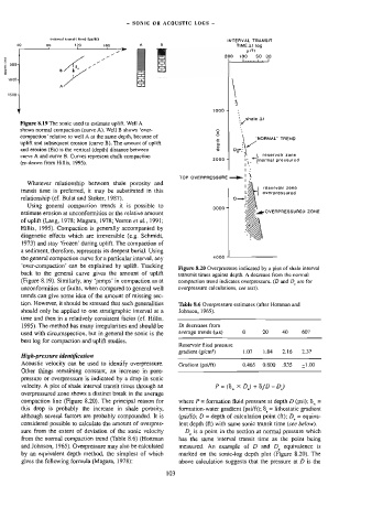
Figure 8.19 The sonic used to estimate uplift. Well A a
z *
shows normal compaction (curve A), Well B shows ‘over-
compaction’ relative to well A at the same depth, because of = ‘NORMAL’ TREND
uplift and subsequent erosion (curve B). The amount of uplift
3 a“
and erosion (Ea) is the vertical (depth) distance between o Os:
curve A and curve B. Curves represent chalk compaction reservoir zone
2000 5 +} normal pressured
(re-drawn from Hillis, 1995). ‘-
TOP OVERPRESSURE
Whatever relationship between shale porosity and
reservolr zone
transit time is preferred, it may be substituted in this ovarpressured
relationship (cf. Bulat and Stoker, 1987).
Using general compaction trends it is possible to
3000 7
estimate erosion at unconformities or the relative amount Ye OVERPRESSUREO ZONE
of uplift (Lang, 1978; Magara, 1978; Vorren et al., 1991;
Hillis, 1995). Compaction is generally accompanied by
diagenetic effects which are irreversible (e.g. Schmidt,
1973) and stay ‘frozen’ during uplift. The compaction of
a sediment, therefore, represents its deepest burial. Using
the general compaction curve for a particular interval, any 4000 ~
‘over-compaction’ can be explained by uplift. Tracking
Figure 8.20 Overpressure indicated by a plot of shale interval
back to the general curve gives the amount of uplift transmit times against depth. A decrease from the norma)
(Figure 8.19). Similarly, any ‘jumps’ in compaction as at compaction trend indicates overpressure. (D and D. are for
unconformities or faults, when compared to general well overpressure calculations, see sex).
trends can give some idea of the amount of missing sec-
tion. However, it should be stressed that such generalities Table 8.6 Overpressure estimates (after Hottman and
should only be applied to one stratigraphic interval at a Johnson, 1965).
time and then in a relatively consistent facies (cf. Hillis,
1995). The method has many irregularities and should be Dt decreases from
used with circumspection, but in general the sonic is the average trends (ws) 0 20 40 60?

best log for compaction and uplift studies.
Reservoir fliud pressure
gradient (g/cm?) 1.07 184 2.16 2.37
High-pressure identification

Acoustic velocity can be used to identify overpressure. Gradient (psi/ft) 0.465 0.800 935 ~1.00
Other things remaining constant, an increase in pore-
pressure Or overpressure is indicated by a drop in sonic
velocity. A plot of shale interval transit times through an P=(8,X D)+8{D-D)
overpressured zone shows a distinct break in the average
compaction Jine (Figure 8.20). The principal reason for where P = formation fluid pressure at depth D (psi); 8, =
this drop is probably the increase in shale porosity, formation-water gradient (psi/f); 8, = lithostatic gradient
although several factors are probably compounded. It is (psi/ft); D = depth of calculation point (fi); D, = equiva-
considered possible to calculate the amount of overpres- lent depth (ft) with same sonic transit time (see below).
sure from the extent of deviation of the sonic velocity D_ is a point in the section at nofmal pressure which
from the normal compaction trend (Table 8.6) (Hottman has the same interval transit time as the point being
and Johnson, 1965). Qverpressure may also be calculated measured. An example of D and D_ equivalence is
by an equivalent depth method, the simplest of which marked on the sonic-log depth plot (Figure 8.20). The
gives the following formula (Magara, 1978): above calculation suggests that the pressure at D is the
103