Page 122 - The Geological Interpretation of Well Logs

- THE GEOLOGICAL INTERPRETATION OF WELL LOGS ~

time (ms)
1 2 3 4

St

8.0_

6.05 P
4.04 <=
44
(km/s}
(ft) pR =
offset velocity 2.04 St <u

=
Measvred Velocities (km/s): SSS
—S

4.4
1.0 : 1 T time (ms} 2 T 3 T
2.95
pseudo-Rayleigh
13
1.47
Stoncley

A. RECEIVER TRACES B. VELOCITY MAP
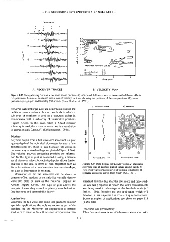
Figure 8.33 Data gathering from an array sonic at one position. A) individual, full-wave receiver traces with different offsets
(i.e. positions). B) dataset combined into a map of velocity vs. time, showing the positions of the compressional (P), shear
(pseudo-Rayleigh, pR) and Stoneley (St) arrivals (from Block er al., 1991).
a) Slowness Track b) Waterfall
However, Schlumberger also use a technique (called the
multishot slowness-time-coherence method) in which a
sub-array of receivers is used as a common gather in
combination with a sub-array of transmitter positions
(Figure 8.32). In this case, when a 5-fold receiver
sub-atay is used, there is an increased vertical resolution
to approximately 0,6m (2ft) (Schlumberger, 1994a).
depth
Displays
=
A typical output from a full waveform sonic too! is a plot
against depth of the individual slownesses for each of the
compressional (P), shear (S) and Stoneley (St) waves, in
the same way as standard logs are plotted (Figure 8.344). 1 I ( J
The velocity analysis processing provides the informa- 60 180
tion for this type of plot as described. Having a discrete slowness (wS/>) = slowness (pS/tth =~
set of slowness values for each depth point allows further
analysis of the data in terms of rock properties such as Figure 8.34 Daia display for the array sonic. a) individual
Poisson’s ratio or other mathematical inter-relationships, slowness logs of discrete, picked values against depth. &)
‘waterfall’ waveform display of illustrative waveforms at
but a lot of information is not used.
selected depths (re-drawn from Smith er al, 1991).
Information on the full waveform can be shown in
constant-offset sections or seismic-like variable density
waveform plots or such as the ‘waterfall display’ of standard borehole log analysis. But more and more stud-
Amoco (Figure 8.346). This type of plot allows the ies are being reported in which the tool’s measurements
analysis of secondary as well as primary wave behaviour are being used to advantage at the borehole scale (cf.
(see fractures and permeability below) Paillet, 1992). Probably the one application which will
develop in this respect is that of detecting open fractures.
Applications Some examples of applications are given on page 113
Generally the full waveform sonic tool produces data for (Table 8.8)
specialist applications: the tools are not run as part of the
standard log set. Moreover, the applications at present -fractures and permeability
tend to have more to do with seismic interpretation than The consistent association of tube-wave attenuation with
112