Page 170 - The Geological Interpretation of Well Logs

- THE GEOLOGICAL INTERPRETATION OF WELL LOGS -

DENSITY
407 SHALE 50
|
|
40
|
307
NEUTRON
% | 30

FREQUENCY 20-4 ~ 20
S
w
3
ra 10

|
“
vi
9 20 40 60 «680 ° 0 0.1 0.2 0.3 0.4 0.5
GAMMA RAY API
LOG ¢ —
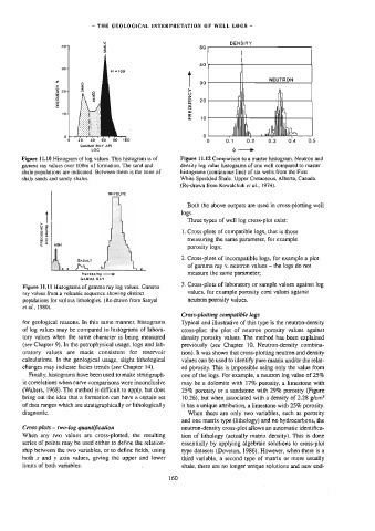
Figure 11.10 Histogram of log values. This histogram is of Figure 11.12 Comparison to a master histogram. Neutron and
gamma ray values over 100m of formation. The sand and density log value histograms of one well compared to master
shale populations are indicated. Between them is the zone of histograms (continuous line) of six wells from the First
shaly sands and sandy shales, White Speckled Shale. Upper Cretaceous, Alberta, Canada.
(Re-drawn from Kowalchuk et ai., 1974).
RHYOUTE

Both the above outputs are used in cross-plotting well
logs.
Three types of well log cross-plot exist:
> |
g2
we 1. Cross-plots of compatible logs, that is those
29
of measuring the same parameter, for example
a 8
acct
uw ASH
porosity logs;
SASALT 2. Cross-plots of incompatible logs, for example a plot
of gamma ray v. neutron values — the logs do not
L
JM,
o_o

measure the same parameter;
inc¢reasing ———»
GAMMA RAY
3. Cross-plots of laboratory or sample values against log
Figure 11.11 Histograms of gamma ray log values. Gamma
values, for example porosity core values against
ray values from a volcanic sequence showing distinct
populations for various lithologies. (Re-drawn from Sanyal neutron porosity values.
et ai., 1980).
Cross-plotting compatible logs
for geological reasons. In this same manner, histograms Typical and illustrative of this type is the neutron-density
of log values may be compared to histograms of labora- cross-plot: the plot of neutron porosity values against
tory values when the same character is being measured density porosity values. The method has been explained
(see Chapter 9). In the petrophysica] usage, logs and lab- previously (see Chapter 10, Neutron-density combina-
oratory values are made consistent for reservoir tion). It was shown that cross-plotting neutron and density
calculations. In the geological usage, slight lithological values can be used to identify pure matrix and/or the relat-
changes may indicate facies trends (see Chapter !4). ed porosity. This is impossible using only the value from
Finally, histograms have been used to make stratigraph- one of the logs. For example, a neutron log value of 25%
ic correlations when curve comparisons were inconclusive may be a dolomite with 17% porosity, a limestone with
(Walters, 1968). The method is difficult to apply, but does 25% porosity or a sandstone with 29% porosity (Figure
bring out the idea that a formation can have a certain set 10.26), but when associated with a density of 2.28 g/cm?
of data ranges which are stratigraphically or lithologically it has a unique attribution, a limestone with 25% porosity.
diagnostic. When there are only two variables, such as porosity
and one matrix type (lithology) and no hydrocarbons, the
Cross-plots — two-log quantification neutron-density cross-plot allows an automatic identifica-
When any two values are cross-plotted, the resulting tion of lithology (actually matrix density). This is done
series of points may be used either to define the relation- essentially by applying algebraic solutions to cross-plot
ship between the two variables, or to define fields, using type datasets (Doveton, 1986). However, when there is a
both x and y axis values, giving the upper and lower third variable, a second type of matrix or more usually
limits of both variables. 160 shale, there are no longer unique solutions and new end-