Page 171 - The Geological Interpretation of Well Logs

- LITHOLOGY RECONSTRUCTION FROM LOGS -

and matrix 100% (matrix point, i.e. for limestone, neu-
tron porosity 0%, bulk density 2.7 g/cm*). Any point on

the plot now has a precise value of the three variables.
This ‘shale point’ cross-plot has many drawbacks.
Firstly, only one matrix can be considered at a time. A
zone will be interpreted as only shaly sandstone or only

shaly limestone — never both. But more importantly. it

mixes definable with undefinable values. Shale is
inevitably very variable, and the shale point therefore
very imprecise (Figure 11.13) yet the matrix and liquid

points are both quite precise (Doveton, 1994). This mix-
ing of precise and imprecise is a general criticism of most
A more realistic approach from a geological point of
shale point cross-plot use.
| view is to define fields of values on this plot in which a
particular lithology is likely to be plotted. The approach
9 19 20 39 40 50 80 79 89 90 100
is empirical and the log limits of each lithological field
NEUTRON POROSITY %
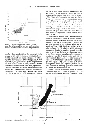
Figure 11.13 Shale point defined on a neutron-density will vary from well to well, and even within one well
cross-plot. Values from 200m of a sand- shale formation. with depth (Figure 11.14). This is best achieved today by
Note the arbitrary choice of one ‘point’ to represent shale.
using software (i.e. TerraStation) which allows the
interactive exploration between logs and their cross-plot,
both of which are displayed simultaneously on the
member values must be defined. For example, to find a screen. That is, intervals selected on the log traces may be
solution for any point when shale is present, a shale end- inter-actively matched to points on the cross-plot (i.e.
member with density and neutron values must be defined. calcareous shale, Figure 11.15) or a set of points on the
Typically, this ‘shale point’ is defined empirically. A great cross-plot identified in their position on the log traces (i.e.
many lithologically unidentified points are plotted and gas sand, Figure 11.15}. Core data may be integrated.
the ‘shale point’ is chosen to correspond to the extreme This approach allows for a rigorous graphical use of
value but within the supposed shale field (Figure 11.13). cross-plots and an effectively quantitative identification
Once the ‘shale point’ is defined, the cross-plot can be of lithology. An extremely useful tool.
divided into a compositional triangle, the end-members A sophistication of the cross-plot method of lithologi-
being shale 100% (shale point), porosity 100% (fluid cal quantification is to cross-plot cross-plots. This is the
point, i.e. neutron porosity 100%, bulk density 1.0g/cm*) basis of the Schlumberger M/-N plot (Burke et ai., 1969).

|
T
!
1.090
|
|
1.80 |
GOAL

o ORGANIC
§ SHALE

& decreasing organics

z 2.00
a
z
w
3 /
s SHALE
/ increasing silt
a

2,60
porous === SILT ~ Pron-porous

T
t
3.00
T
0 10 20 30 40 60 60 70 80 90 100
NEUTRON POROSITY %
Figure 11.14 Lithological fields defined on a neutron-density cross-ptot. Based on the values from a 500m interval in one well.
161